
You have sent an Excel sheet to a co-worker for revision and received it back. The problem: You don’t know what has changed. Here is how to compare two Excel sheets.
Introduction
Comparing two worksheets and seeing the differences is probably one of the most common and most troublesome tasks in Excel. And admittedly, no method is perfect. In this article, I describe four different methods. You should then use the one that is most suitable for you.
Example in this article
The example: You have an “original” worksheet and one “revised”. On the revised sheet somebody has changed cells – and you don’t know what has changed.
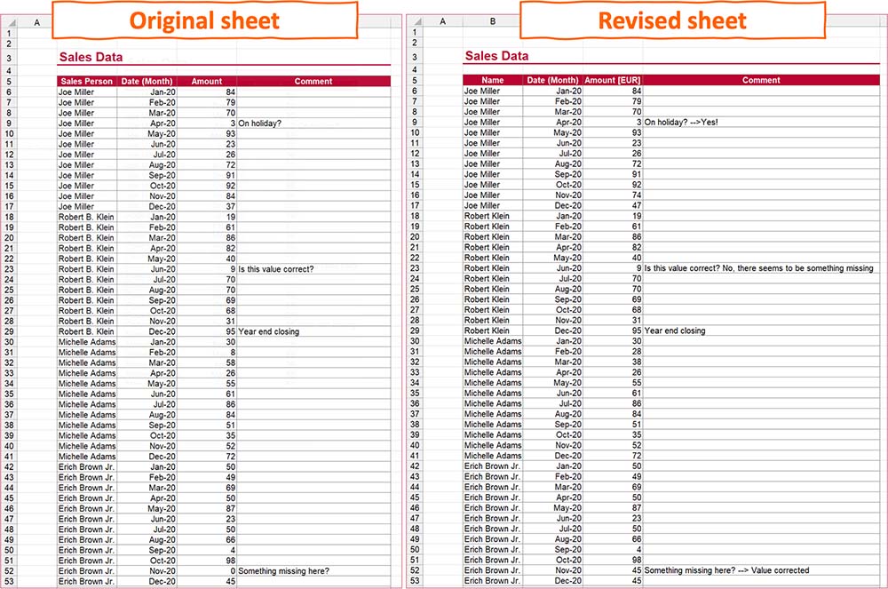
We separate the following four methods into two different approaches. The first approach (in the following called Approach A): The structure of both worksheets (original and revised) is exactly the same. No changed columns or rows, nothing sorted etc. This approach is usually easier because you can compare cell by cell.
The second approach is more complicated but unfortunately more common: We use it when the structure of rows and columns is not the same or somebody has been sorting the table.
Approach A: Compare cell by cell
Method A1: Compare cell by cell with Excel formula
This method is quite straight-forward. You just compare cell by cell, using a simple Excel formula. Already the following version would return the desired result. Just copy it into a new worksheet in cell A1 and pull it down and to the right.
=Original_Sheet!A1=Revised_Sheet!A1 The formula returns either TRUE if the cell content is equal or FALSE if not. Simple, right?
We can further modify it so that we also return the differences:
=IF(Original_Sheet!A1=Revised_Sheet!A1,"","Original: "&Original_Sheet!A1&CHAR(10)&CHAR(10)&"Revised: "&Revised_Sheet!A1)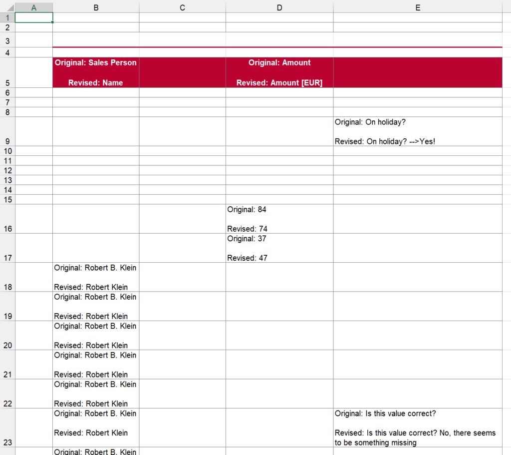
Advantages
- Comparatively simple (one Excel formula to enter).
- Good for a first overview.
Disadvantages
- Does not work if the sorting has changed.
- Has problems, when rows or column are added or removed because all following rows and columns show differences.
- When differences show up, investigation of what has really changed might be troublesome.
Method A2: Compare two sheets with an Excel add-in
To provide some more convenience, we have included a comparison feature in our Excel add-in Professor Excel Tools.
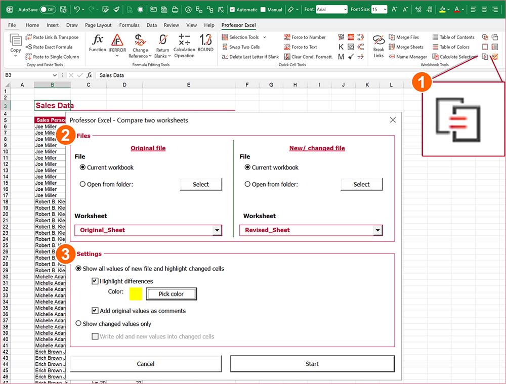
- Just click on the Compare Sheets button on the Professor Excel ribbon.
- Select the sheets you would like to compare. Also possible: Use sheets from other workbooks (for example when you revised / updated version is open and the original worksheet is saved on your hard drive).
- How do you want to compare the two worksheets? You can define in detail: Show all values from the updated version and highlight the changes or only show the cells that have changed.
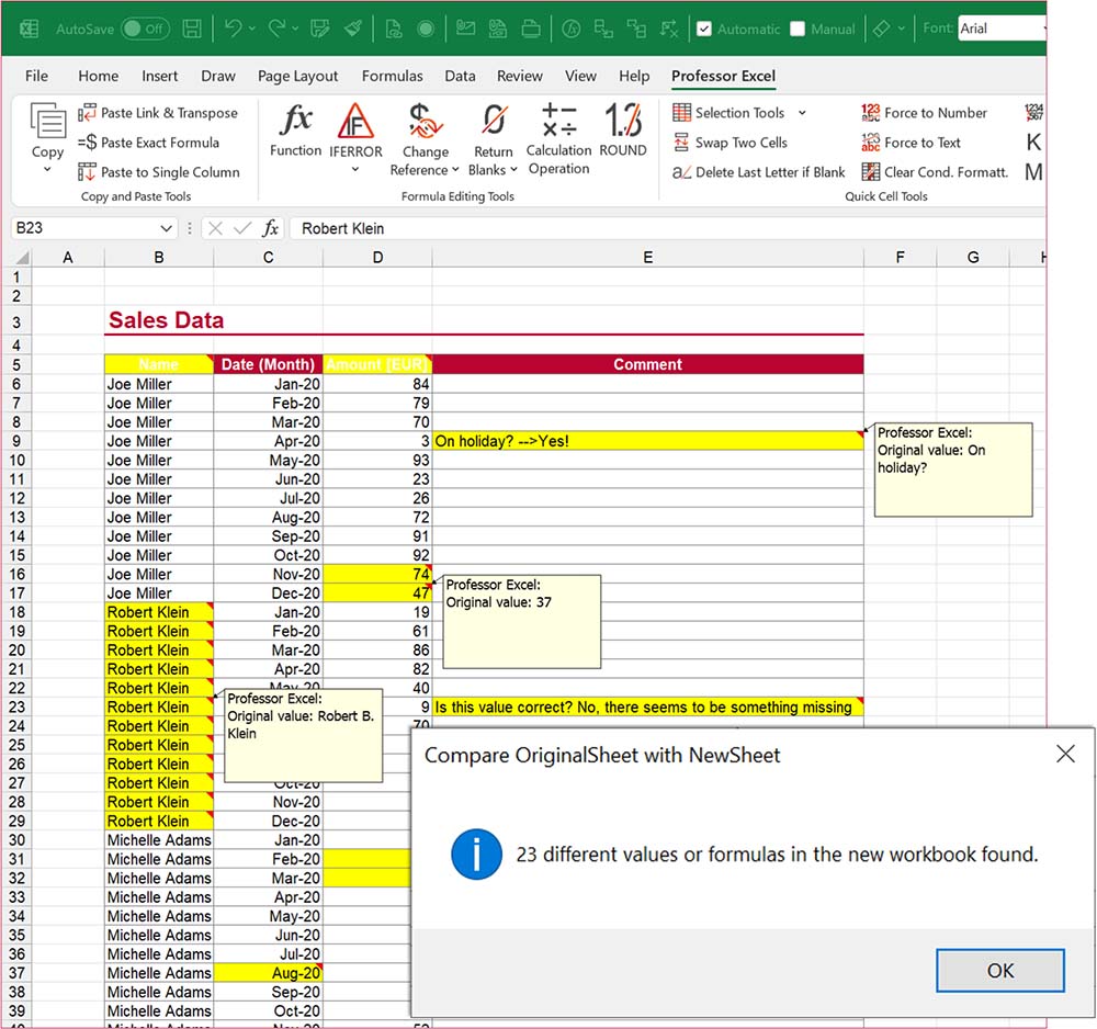
The results (depending on the settings), look like this:

This function is included in our Excel Add-In ‘Professor Excel Tools’
(No sign-up, download starts directly)
More than 35,000 users can’t be wrong.
Approach B: Content-wise comparison – compare two lists (also, if sorting has changed)
Our second approach is much more complex than the first one. But: It regards differently sorted lists and tables as well as different column structures (order and names).
Method B1: See differences of two simple lists
Let’s take a look at an easier example: You have two lists and want to know which items are in both lists, and which item is only available in one of the lists.
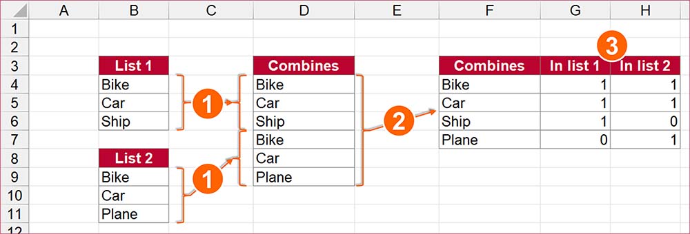
- First, set up a comparison table. This might as well be an additional worksheet. The first column will later on contain the whole list. The following columns will show, if the item is available in the lists.
So, in order to compile a lists with all items, first copy both lists completely underneath each other. - Next – as many items might occur two times in our combined list – we need to remove duplicates. Excel provides a (very useful) function, called “Remove Duplicates”. Therefore, select the whole list and go to Data and click on Remove Duplicates.
- As the last step, we count how often each item occurs in each list. In our example, the formula in cell G4 would be “=COUNTIFS($B$4:$B$6,$F4)”. Do it the same way in column H for the second list. If you need assistance with the COUNTIFS function, please refer to this article.
There are probably also other methods to compare two lists, but these steps should be comparatively easy.
Method B2: Use our comparison Excel template (free download)
Now, we are coming to the most complex method to compare two tables. It can deal with different structures and changed rows (sorted, etc.).
Requirements:
- The tables must have a primary key. A primary key is able to identify each data entry. It might also be a combination of several columns as you will see in the example.
- Your tables must have headlines which can identify the columns.
To allow such complex comparison, I have created a template. This template should be fairly easy to use.
How to use our comparison template
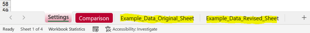
The template has two comparison worksheets:
- Sheet “Settings”: On the sheet Settings you have to fill in the basic settings, including both sheet names (of the original and revised worksheets) and in which row and column the data starts.
- The actual comparison takes place on the sheet “Comparison”. You don’t have to change anything here.
Start by copying your two worksheets into this template (you can of course remove the example data sheets) like in this example:
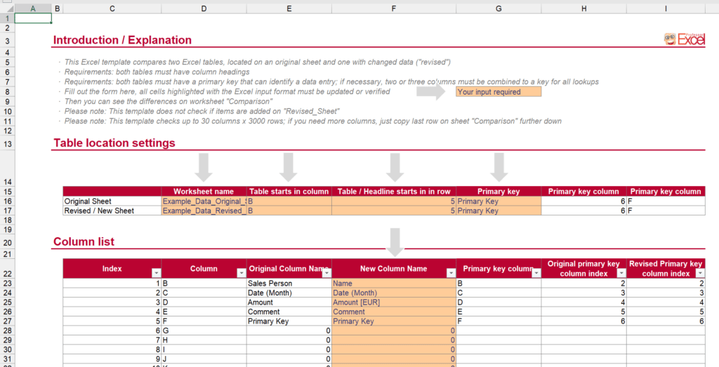
Basic comparison settings on Sheet “Settings”
On the sheet settings you have to define the basic settings, separated into two parts: Table locations (where are the two tables located with sheet name, first row, first column and the primary key column). The lower part has the column list in which – in case sequence or names of the columns have changed – you check and if necessary correct the column mapping.
The sheet has detailed instructions so I am not going much further here.
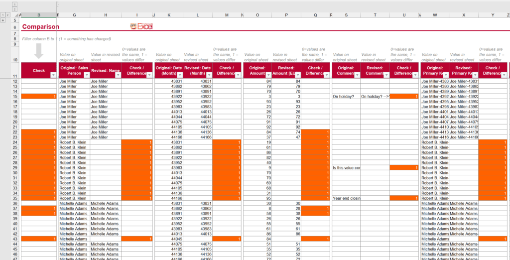
How to understand the comparison results
Once you have filled in the settings, go to the second sheet to see the result. Nothing to fill in here, but filter column B to “1”. 1 means that something has changed. You can see the comparison column by column – all changes are highlighted in orange.
Download the Excel template
Please feel free to download the template here:
Image by Martin Pyško from Pixabay