Quick Access Toolbar in Excel: Everything You Need to Know

You probably know this situation: You just quickly want to use a function in Excel, but it takes you way too much time searching it within the menu bar. Admittedly, the ribbon structure of Excel can be quite confusing. But there is a solution: The Quick Access Toolbar. You can save the most important or frequently used buttons in this menu bar on top of the screen. That way, you can easily access your favorite functions. So let’s see how it works and learn some tips and tricks.

Please note: There will be updates end of 2021 for all Microsoft 365 subscribers (formerly Office 365). While most things remain the same, the layout slightly changes and a few buttons might be relocated. Please refer to this article for the upcoming changes.

The Ribbon

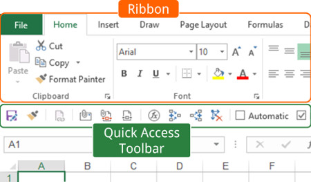
First of all, what is the Ribbon and what is the Quick Access Toolbar?

Excel is organized within two major menus:

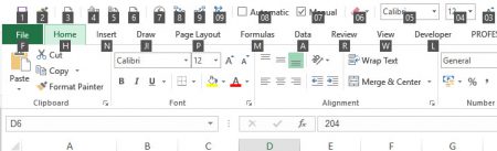
1. The Ribbon, the large menu bar on top of the worksheet.
2. You can add buttons (which you frequently use) to the Quick Access Toolbar (QAT). The QAT is a small row of button above or below the ribbon.

Using these two menus cleverly, you can save a lot of time. Let’s take a close look at it.

The Quick Access Toolbar

The “QAT” is always on top of the screen. It doesn’t change when you go to another ribbon. That’s why it’s very useful: You can save your most important functions there and always “quickly” access them.

Add or remove buttons to the Quick Access Toolbar

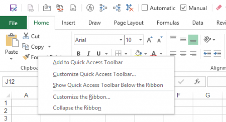
Adding and removing buttons from the QAT is very easy: Just right click on any button on the ribbon and click on “Add to Quick Access Toolbar”. Yes, it’s that simple. If the button is greyed out it means that it is already in your “QAT”.

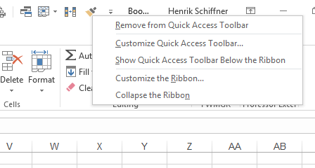
Removing a button works almost the same way: Right click on the button on the “QAT” and click on “Remove from Quick Access Toolbar”. Now it’s gone again.

How to organize the Quick Access Toolbar

Often, you slowly add more and more button to the Quick Access Toolbar. After some time, you might want to reorganize it or clean it up.

Excel offers a menu for (re-)moving button to the Quick Access Toolbar. You can also add more rare (but still very useful buttons), which are not on any ribbon.

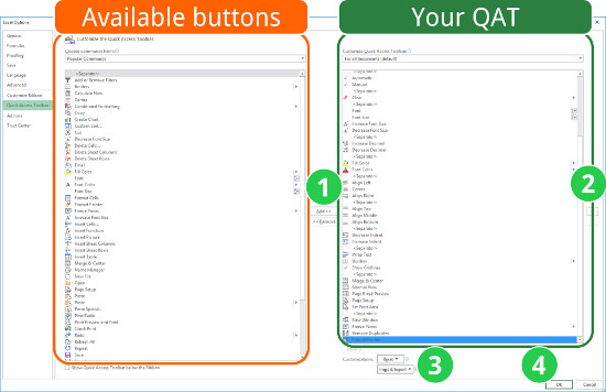
Right click on the Quick Access Toolbar. Then click on “Customize Quick Access Toolbar”. Now you will see the window on the right side. It has to parts: The available commands (orange) and your current Quick Access Toolbar (QAT, green).

You got the following options (the numbers correspond to the picture):

1. Add or remove buttons. Select a button on the left hand side and press add. It will be inserted into your Quick Access Toolbar right under your currently highlighted item.
   If you want to add a special button, change the drop-down menu on the top from “Popular commands” to “All commands”.
2. Move your buttons up or down with the small arrow buttons in order to re-organize their order.
3. Furthermore, you can import or export existing Quick Access Toolbar. Attention: If you import such settings, the existing customization will be lost.
4. Confirm by clicking OK.

Import and export customization files

Please take a look at the image above: Importing and exporting customization files can be done by clicking that button. These customization files include your current Quick Access Toolbar settings as will as your personal ribbon settings (if you got some).

How do you get there? Right click on any ribbon or your Quick Access Toolbar and click on “Customize Quick Access Toolbar”.

Attention: If you import such settings, the existing customization will be lost.

Add a button for a VBA macro

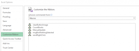
Besides normal buttons you can also create buttons for your VBA macros. Excel allows you to add any “Sub” with no arguments. “Private Subs”, “Subs” with input arguments or functions don’t work.

In order to add your individual button, right click on the QAT again. Next, click on “Customize Quick Access Toolbar”. Switch the top drop down menu from “Popular commands” to “Macros”. Now you see the list of your available macros (either in your current document or of your Excel add-in (“xlam”-file). Simply add them with the Add button.

How to show the QAT under or above the ribbon

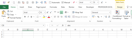
You got two options for the location of the “QAT”: Above or under the ribbon. Both positions have advantages and disadvantages:

	Advantages	Disadvantages
QAT above the ribbon	Needs less space, as the space is otherwise just blank.	Half of the ribbon will be hidden when a new (special) ribbon (like “PivotTable”) opens.
QAT below the ribbon	Won’t be hidden when a new ribbon (like “PivotTable”) opens.	Needs more space on the screen than above the ribbon.

You can easily change the position: Right click on any ribbon or the QAT and click on “Show Quick Access Toolbar above the Ribbon” (or below, depending on the current state).

How to hide the Quick Access Toolbar completely

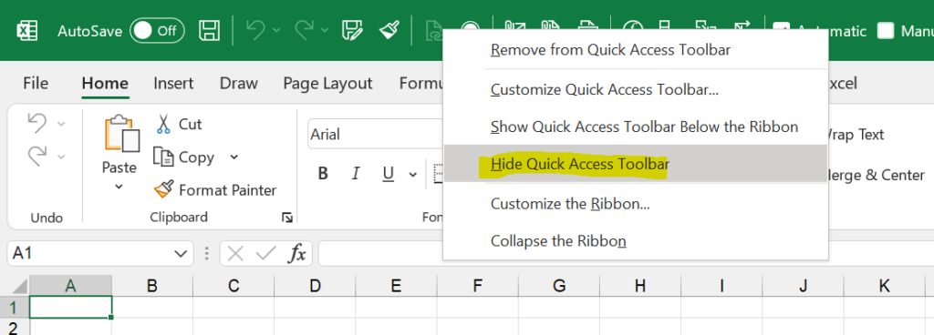
In newer Excel versions, you can hide the QAT completely. Just right-click on it and then on “Hide Quick Access Toolbar”.

You want to get it back? No problem. Now, right-click on any ribbon and then on the “Show Quick Access Toolbar” button.

How to show descriptions / names of the buttons in the Quick Access Toolbar?

Besides the buttons, you can also show the names next to them in the QAT. Just right-click on the QAT and then on “Show Command Labels”.

Hiding the button names works the same way: Right-click on the QAT and then on “Hide Command Labels”.

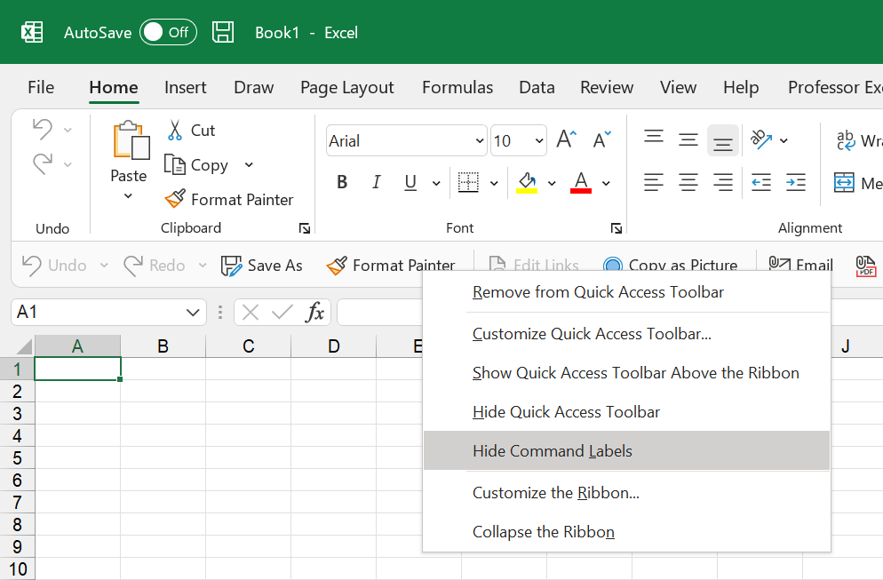
Please note: This only works with newer versions of Excel / Office and only if the QAT is located below the ribbon.

Access the Quick Access Toolbar with keyboard shortcuts

All you have to do is press the Alt key on the keyboard. Excel shows you then your options for accessing the QAT with keyboard shortcuts, usually shown with numbers. The first QAT got the number 1, the second one 2 and so on. Just press it and you can use keyboard shortcuts for your individual QAT. Quite cool, isn’t it?

Which buttons should you add to the Quick Access Toolbar?

The short answer: It depends. It highly depends on what you need in your daily life in Excel and what steps you already got covered with keyboard shortcuts. If you for example always use Ctrl + c for copying cells, it doesn’t make sense to add the copy button to the QAT.

But still, we got some advice for you:

• Slowly add – one by one – button of functions you usually take some time searching for.
• Nonetheless, you should make sure that you sometimes use these commands. Don’t add functions you only use once per year – therefore the space is too precious.
• There are some button with the same functions in all Microsoft Office programs. A good example is the format painter: It is available in Word, PowerPoint, Excel and even Outlook. So why don’t you put it in the same position in each program? That way, you can also remember the corresponding Alt-keyboard shortcut easily.
• Most important shortcuts should go to the left hand side of the QAT. That way, they won’t be covered if a new ribbon opens. Also the keyboard shortcuts for accessing them is shorter and therefore easier.

Download: Our Quick Access Toolbar for your reference

It’s contradicting: In the previous chapter we just said that you should make up your individual “QAT”. But nonetheless, we’ve created an example of what buttons might be useful. But of course, it highly depends on your daily work in Excel.

So this is our suggestion:

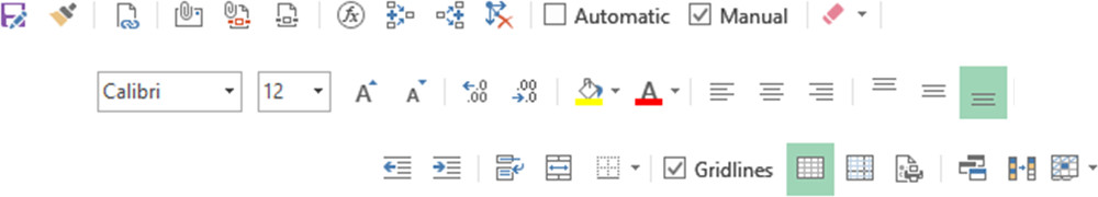
Explanation

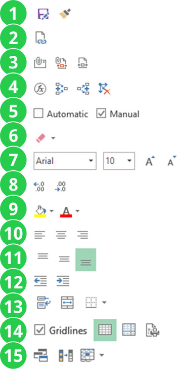
Let’s go through it by groups (each group is divided by a separator):

1. The save-as and format painter buttons we use throughout Microsoft Office. Maybe the save-as button is not really necessary as there is a direct shortcut (just press F12). But the format painter is very useful.
   You might notice, that there is no undo or redo button. The reason is, that we use these functions with the keyboard (Ctrl + z and Ctrl + y).
2. Edit links is for our daily work very helpful. It’s not only a button, it also shows if there are links in the workbook.
3. The third group contains sharing and exporting functions:
   1. Attach the active workbook to a new email.
   2. Attach the active workbook as a PDF file to a new email.
   3. Save the selected worksheets as a PDF file to the disk.
4. These formula auditing buttons are very helpful for error checking: Check the current formula step by step or trace precedents and dependents.
5. Change between automatic and manual calculation. Also these buttons not only let you change the calculation method, they also show you the current option.
6. Clear not only the cell contents but also the formatting with the additional deleting options.
7. All important buttons for the font (type and size).
8. Increase or decrease the number of decimals.
9. These – and the following groups – are about formatting: Fill color and font color.
10. The horizontal text alignment (left, center, right).
11. The vertical text alignment (top, middle, bottom).
12. Increase or decrease the indentation.
13. Further cell formatting options:
    1. Wrap text.
    2. Merge selected cells.
    3. Define the cell borders.
14. Sheet layout options:
    1. Hide or show the gridlines.
    2. Normal view.
    3. Print preview.
    4. Print setup.
15. Miscellaneous:
    1. View current workbook in more windows.
    2. Remove duplicates.
    3. Freeze header rows or columns.

Download

If you like these suggestions, please feel free to download the whole customization file here. You can import it into your Excel as described above. But please be aware, that your current customization will be removed. So please export it first if you want to keep it.

Image by Free-Photos from Pixabay