

In a previous Excel Tip we have learned how to create a simple Excel Pivot Table. Now we will go on from there and learn how to eliminate one of the major pains of Pivot Tables: It changes the size of the columns after each update of the values.
Steps for fixing the column width when updating Pivot Tables
When you change your data, you have to refresh the Pivot Table. Therefore, right-click on any value and click on “Refresh”. Now, the column width adapts to the new data – even if you carefully changed the columns before. To avoid that, do the following steps (the numbers are corresponding to the picture above):

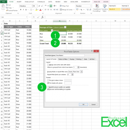
- Right click on any value within your Pivot Table.
- Click on “PivotTable Options”.
- Remove the tick at “Autofit column widths on update”.
That’s it. Now the column width stays the same on each update.
Do you want to know one more very helpful tip about PivotTables? Read here how to disable the “GETPIVOTDATA” when you refer to a PivotTable.