

You have some data and want to gain a quick overview? Or conduct some easy evaluation? Maybe later on analyze the data more detailed? For all these purposes, a Pivot Table can be a good choice.
What does a Pivot Table do?
With Pivot Tables you can summarize your data. Each column of your data is represented by one “data field” having the name of the first row of your data table (the heading row). You can summarize each field by dragging and dropping them into your Pivot Table:
- If you put a data field into the Pivot Table rows, for all the different data within the column of the Pivot Table source, an entry will be created. So you’ll get a list of all possible data in this data field
- The same works for columns: If you drag and drop a data field into the Pivot Table column you’ll get one row for each data unique entry.
- If you put a data field into the center of the table, this column from the source data will be summarized, for example by summing it up or counting it depending on the rows and columns.
How to create Pivot Tables?

- Make sure that your data meets the following conditions: Each column has a unique heading/name and there are no blank columns.
- Select all your data, including the header row.
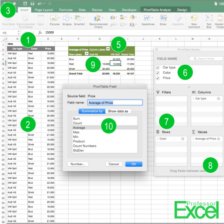
- Click on “PivotTable” on the left hand side of the Insert ribbon.
- Follow the steps shown. Usually, the default settings are fine. You can just skip through the windows.
- Now, an empty Pivot Table will be shown.
- Drag and Drop your data from the field list…
- …to the rows or columns of your Pivot Table.
- Drag the values that you want to summarize (e.g. to sum up) to the “Values” field.
- Right-click on the value in the Pivot Table and then select “Value Field Settings”.
- Select if you want to see e.g. the number of values, sum or average.
In our example, we want to know the average prices of each car type and color. We could as well display the sum of each value.