How to Freeze the Headings

Your worksheet is larger than your screen? When you scroll up and down, the header row of your data is invisible? Then let’s take a look at how you can make the header row or a column stick to the top of the screen (or on the left hand side in case of a column).

 

How to freeze panes

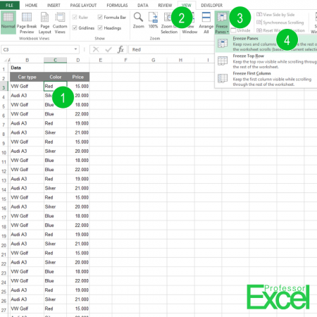
The function in Excel is called ‘Freeze Panes’. Freezing panes helps and keeps the important header row(s) always on top (the numbers are corresponding to the picture on the right hand side):

1. Select the cell, whose the row above and the column on the left you want to freeze.
2. Go to the “View” ribbon.
3. Click on “Freeze Panes”.
4. Click again on “Freeze Panes” on the list.

Now, the rows above and the left columns of your marked cells are frozen.

There are also the options of just freezing the top row of the sheet or the first column.

 

Keyboard shortcuts for freezing panes

If you want to freeze the heading rows or columns faster, you might want to memorize this keyboard shortcut: Type Alt –> w –> f –> f one after another. With this shortcut you either set the or you remove the freezing, depending on if it is set already.