Negative Values in Red Color: 3 Easy Methods for You!

A good Excel table provides a quick overview of the most important facts and figures. One way of highlighting important numbers is by using colors. For example, values below zero should stand out. In this article we’ll explore two ways of highlighting negative values in red color in Excel.

Method 1a: Highlight negative values with cell formatting

The first method for highlighting negative values in red color is quite simple: Changing the number format to the predefined format for red negative numbers.

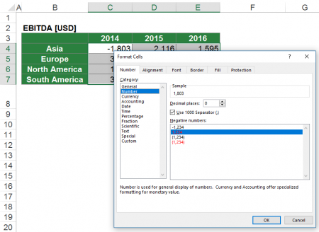
• Right-click on the cell and select “Format Cells…”. Alternatively, press “Ctrl + 1” on the keyboard.
• On the “Number” tab, select the category “Number” and change the format to the second or fourth option (negative numbers have red color and the “-” sign is shown). 

Method 1b: Use a custom cell format

The first method (1a) above has one disadvantage: It removes the minus sign for negative values. If you want to keep it, you can easily tweak it:

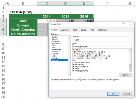
• Proceed as written in the method 1a above (set the cell format to Number and choose the second option).
• Click on “Custom” on the left hand side. Add the minus sign as shown in the image above or copy the following code:
  #,##0;[Red]-#,##0  
  Paste it into the “Type” field in the center of the window.
• Confirm with OK.

Method 2: Use conditional formatting for highlighting negative values

The second method is a little bit more complicated but offers more options: Use conditional formatting.

Conditional Formatting allows you to set formats, symbols and even small bars within the cell depending on the values. Follow these steps to set up a conditional format for highlighting negative numbers:

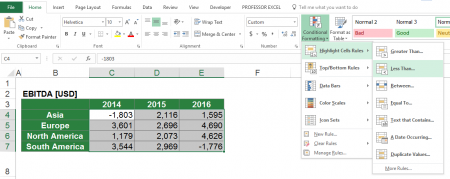
• On the Home ribbon, click on “Conditional Formatting” and then on “Highlight Cells Rules…”.
• Click on “Less Than”.

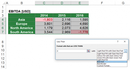
Now you’ll see a small pop up window as shown on the right hand side.

• In the left text field type 0 because you want to format all negative values.
• Now you can select a predefined style (for example the “Light Red Fill with Dark Red Text” like on the screenshot. Or just choose the “Red Text” option. You can also set a custom format with the last entry.

For more information about how to use small symbols or shades of the background color, please refer to this article. This article provides more information of how to use conditional formatting with formulas. 

Bonus Tip: Remove conditional formatting rules but keep the colors

In some cases, you want to remove the conditional formatting rules but keep the format. For example, you’ve selected the background color depending on the values (see above). Now you want to keep the color, but either delete the values or even change the values.

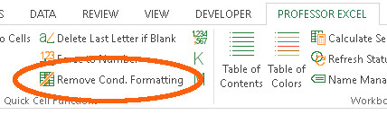
There is one very comfortable way: Use “Professor Excel Tools“:

1. Select the cells having conditional formatting rules.
2. Click on “Remove Cond. Formatting” within the Quick Cell Functions on the Professor Excel ribbon.

You can try the Excel add-in for free – no sign-up or installation needed. Just click the button below.