


You have finished your calculations and now you are about to present your results? Well built Excel models usually separate the calculations from the results. Therefore “Paste Links” might be helpful for you, especially when your colleagues should not mess your data source.

This article describes how to paste links to cells instead of values and the next steps for also applying formatting with just a few klicks (or better: key strokes…).
How to paste links instead of values
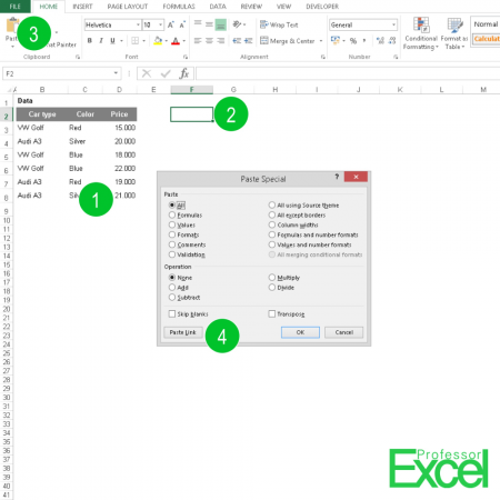
Pasting links to the source cells instead of values or formulas is quite easy and Excel offers this option within the paste special window. The following number are corresponding to the picture above:

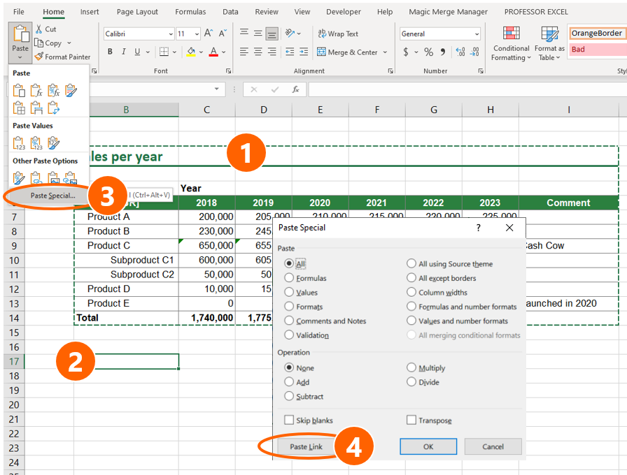
- Instead of working with the original data, you could just link to it by copying it with “Ctrl + c”.
- Select the cell which you want to paste the copied cells as a link.
- Instead of pasting it now with “Ctrl + v”, paste it using “Ctrl + Alt + v” (Paste Special).
- Click on “Paste Link”.
In case of large Excel models, it’s recommended doing this with a new Excel worksheet, so that your results are really separated from the calculations. As your data is linked to your original source, you can edit the original source as usual and the linked table refreshes automatically. Instead of sending your original data to others, you now only send the new sheet.

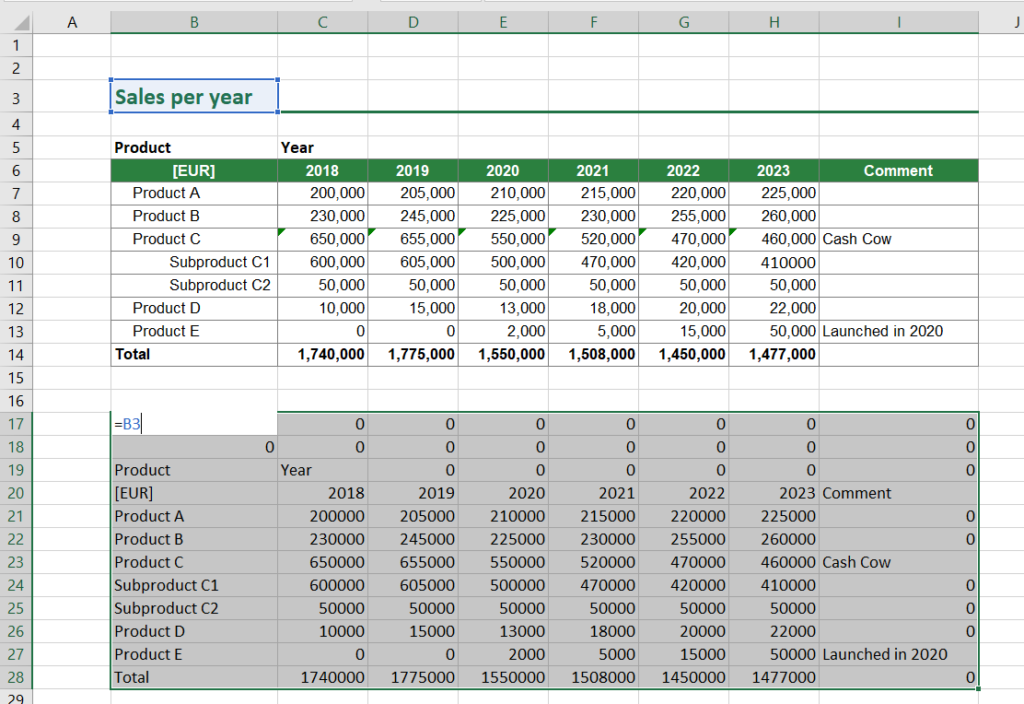
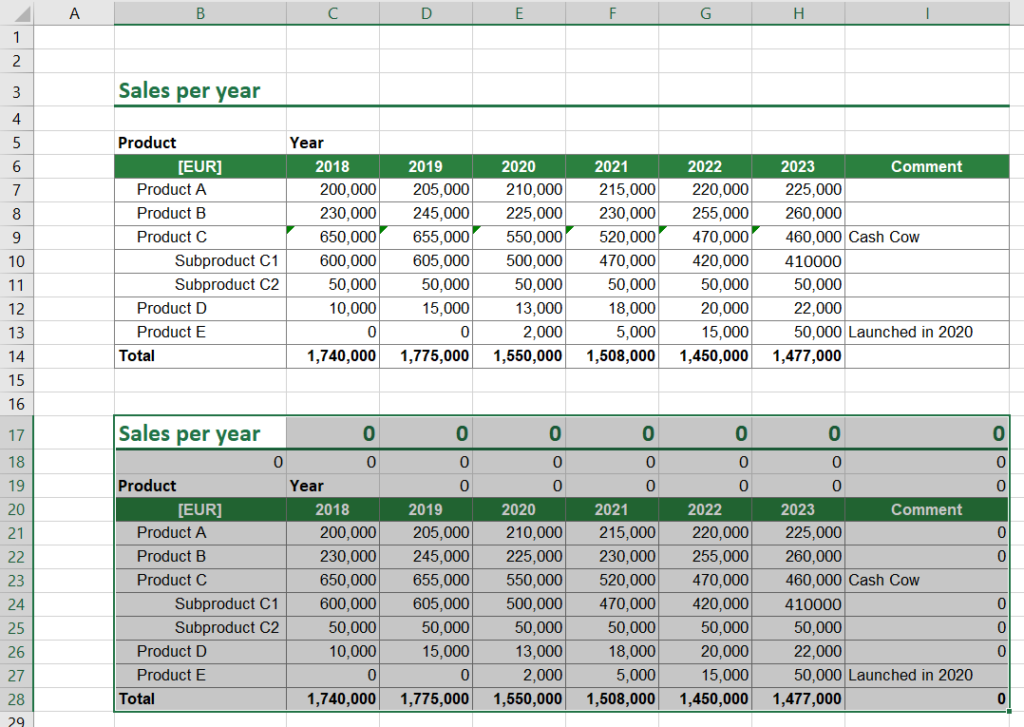
Result: This is, how the paste links function looks like:
Next step: Don’t only paste links but also the formatting
After you have inserted simple links, you can next also paste the formatting. That way, the pasted cells look like your original cells.

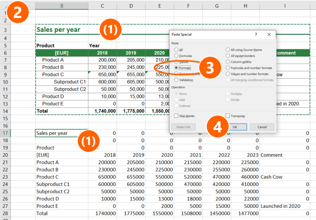
The good thing is that usually your original cells are still copied. So, before you click anywhere or type anything, simply re-do the paste special. Instead of pasting links, you paste the formatting this time.
- (Just, if your original cells aren’t copied any longer. So, the big green, dashed borders are gone): Copy the original cells again. Also, select the target cell.
- Open the paste special window again. Either click on the small arrow of the Paste button on the Home ribbon (on the far left) or simply press Ctrl + Alt + V on the keyboard.
- Select “Formats”.
- Click on “OK”.

That’s it, your cells should look something like this.
And the last step: Hide zeroes
Admittedly, that doesn’t look perfect yet. The zeroes bother me. You can choose between different approaches:
- Hide zero values: Please refer to this article.
- Delete all zeroes. Therefore, select all zeroes and press Del on the keyboard.
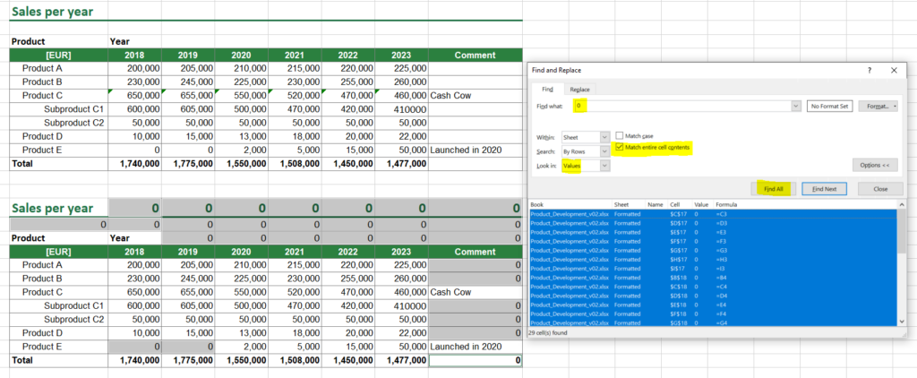
In case you have inserted a lot of links to blank cells, you might want to use the Search function in Excel to select all zeroes:

Do you want to boost your productivity in Excel?
Get the Professor Excel ribbon!


Add more than 120 great features to Excel!
One more example: Link to non-coherent cells
Very practical: You don’t have to use coherent cell ranges. You can also select and copy separate ranges of cells:

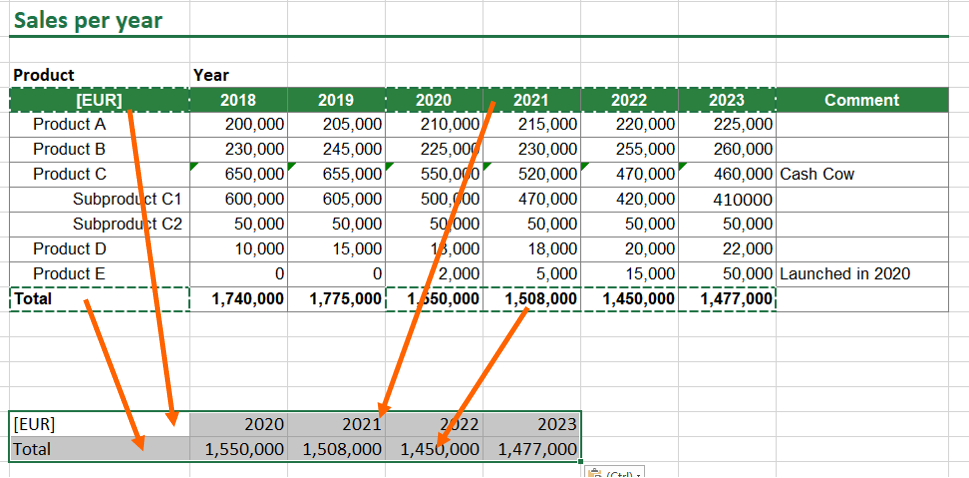
One limitation: Your copied cell ranges must have the same shape.
Convert absolute to relative references: Insert $-signs to all formulas
Thanks for the question in the comments below! The question was how to insert $-signs to all pasted cell links. Because this question would be relevant in many different scenarios (not only when pasting cell links), I’ve written a whole article about it. The short answer: Use a VBA macro to insert $-signs to all cell references.
Please read this article for more information.
Image by Денис Марчук from Pixabay