


Sometimes Excel workbooks become quite large: The more worksheets there are, the more difficult it is to keep the overview. A table of contents might help. In this article we’ll explore 4 ways of creating tables of contents in an Excel workbook.
Let’s say, we want to create a new worksheet with a list of all other worksheets. Furthermore, each list entry should have a link to the corresponding worksheet so that you can easily click on it and will be taken to this worksheet at once. Basically, there are four methods for creating such table of contents: Do it manually, apply a complex formula, use a VBA macro or an Excel add-in.
Method 1: Create a table of contents manually

The first method is the most obvious one: Type (or copy and paste) each sheet name and add links to the cells. These are the necessary steps:
- Create a new worksheet by right clicking on any worksheet name and click on Insert Sheet (or press Shift + Alt + F1). Give a proper name, for example ‘Contents’.
- Start by typing the first worksheet name into cell B4 (or any cell you like…).
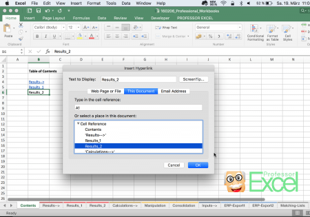
- Add the link to the cell: Right click on the cell and click on ‘Hyperlink’. Select ‘This document’ as shown on the picture above and click on the sheet name you want to create the list entry for. Usually cell A1 is fine as the cell reference. The window of adding a hyperlink on Windows looks a little bit different but offers the same options.
- Repeat steps 2 and 3 until all worksheets are in your table of contents.
- Do all the formatting as desired and then you are done.
Method 2: Use formulas for a table of contents

Thanks to Brian Canes, who posted this method as a comment: There is actually a way of using formulas and named ranges. Follow these steps:
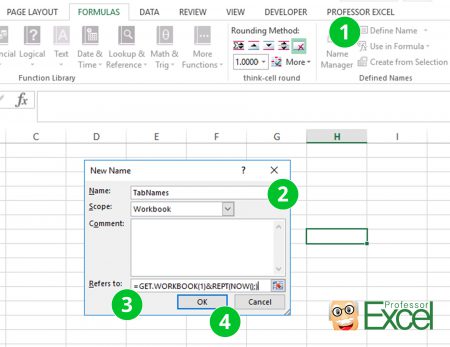
- Click on “Define Name” in the center of the Formulas ribbon.
- Type the name “TabNames”.
- Copy and paste this code into the “Refers to:” field: =GET.WORKBOOK(1)&REPT(NOW(),)
- Confirm with OK.
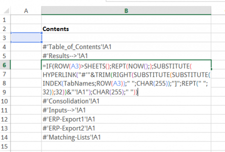
- Copy this formula into any cell. As it refers to the cell A1, it’ll be the entry for the first worksheet in your workbook:
=IF(ROW(A1)>SHEETS(),REPT(NOW(),),SUBSTITUTE(HYPERLINK("#'"&TRIM(RIGHT(SUBSTITUTE(SUBSTITUTE(INDEX(TabNames,ROW(A1))," ",CHAR(255)),"]",REPT(" ",32)),32))&"'!A1",TRIM(RIGHT(SUBSTITUTE(SUBSTITUTE(INDEX(TabNames,ROW(A1))," ",CHAR(255)),"]",REPT(" ",32)),32))),CHAR(255)," "))

- Copy this formula down until you get blank cells.
Please note:
- All worksheets will be regarded, also hidden ones.
- If you change the order of worksheets, delete some or do any other changes: These changes will be immediately reflected in the table of contents. So you have to be careful if you add comments or do any special formatting.
- You have to save the workbook as a macro enabled workbook in the format “.xlsm”. The reason is that you use a formula as a named range which is only possible with macro-enabled workbooks.
Do you want to boost your productivity in Excel?
Get the Professor Excel ribbon!


Add more than 120 great features to Excel!
Method 3: Use a VBA macro
As the first two methods works but is quite troublesome – especially for large workbooks – we’ll take a look at a third method: A VBA macro. The macro is supposed to do the same steps: Walk through all sheets, create a list entry for each sheet and insert a hyperlink to each sheet.
- Go to the developer ribbon.
- Click on “Editor”.
- Add a new module.
- Paste the following code.
- Press start on the top.
Sub insertTableOfContents()
    Dim PROFEXWorksheet As Worksheet
    Dim tempWorksheetName, tempLink, nameOfTableOfContentsWorksheet As String
    Dim i As Integer

    'Add a new worksheet
    Sheets.Add

    'Rename the worksheet
    nameOfTableOfContentsWorksheet = "TableOfContents"
    ActiveSheet.Name = nameOfTableOfContentsWorksheet

    'Add the headline
    Range("B3") = nameOfTableOfContentsWorksheet

    'Initialize the counting variable i
    i = 0


    'Go through all worksheets as described
    For Each PROFEXWorksheet In Worksheets
            'Copy the current worksheet name
            tempWorksheetName = PROFEXWorksheet.Name

            'Create the link from the current worksheet and link it to cell A1
            tempLink = "'" & tempWorksheetName & "'!R1C1"

            'Add the list entry
            Sheets(nameOfTableOfContentsWorksheet).Cells(i + 5, 2) = tempWorksheetName

            'Select it for inserting the hyperlink
            Sheets(nameOfTableOfContentsWorksheet).Cells(i + 5, 2).Select

            'Insert the hyperlink
            ActiveSheet.Hyperlinks.Add Anchor:=Selection, Address:="", SubAddress:=tempLink

            'Proceed with next entry and increase i therefore
            i = i + 1
    Next
End Sub
Method 4: Use an Excel add-in to create a table of contents

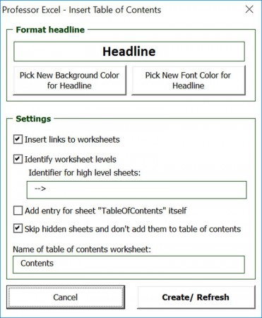
There are some Excel add-ins for creating a table of contents. We – of course – recommend our own add-in. It doesn’t only insert a table of contents but you can easily customize it:
- You can customize the headline color.
- You can choose if you want to insert links to each worksheet.
- You can define levels: For example by high level sheets by their name.
- You can select if you want to insert an entry for the table of contents sheet itself.
- You can choose if you want to skip hidden worksheets or include them as well.
- You can define your preferred name for the table of contents sheets.
Your last settings will be saved so that it’s very fast to update or create a table of contents. There is a free trial version with no sign-up available. Click here to start the download.


This function is included in our Excel Add-In ‘Professor Excel Tools’
(No sign-up, download starts directly)
More than 35,000 users can’t be wrong.