


When you copy and paste cells in Excel, you can either paste them as links or transpose them. Excel doesn’t allow doing both at the same time. Unfortunately, you often need to link and transpose. But there are three ways for accomplishing this: Doing it manually, using the array formula {=TRANSPOSE()} or Professor Excel Tools.
The problem: “Paste Link” button is greyed out

You’ve copied a range of cells. Now you want to paste them. But instead of simply pasting them you also want to paste links and transpose (exchange rows and columns) them.
The problem: As soon as you set the tick at “Tranpose”, the “Paste Link” is greyed out.
Method 1: Use the OFFSET function

The OFFSET function is powerful but unfortunately especially for beginners not very easy to use. Roughly said, you define a base cell and tell Excel which value counting from the base cell to return.
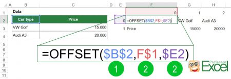
First: Prepare the number 0-2 (the maximum number of rows – 1) on the top and 0 to 1 on the left hand side. We use this as a reference. There are certainly more elegant ways (e.g. with ROW() or COLUMN()) but this is the fastest and easiest method. The following number match to the picture above:
- In our case, the base cell is the left top corner cell of the range we want to transpose and link. This base cell should not change when we copy and paste the formula so that we insert the $-signs.
- The second part of the OFFSET formula defines, how many rows your target cell is away from the base cell. We want this number to increase when we pull the formula to the right hand side. That’s why we don’t add a $-sign in front of the column (“F”). But when copying down the formula, the first row should be fixed with a $-sign.
- Similar for the columns: When we pull down the formula, we want the column index to increase. That’s why we fix the column but not the row.
The formula in the example above looks like this:
=OFFSET($B$2,F$1,$E2) Method 2: Array formula “TRANSPOSE”

With an array formula you don’t have to drag and drop cells manually. Despite the advantage of not having to do anything manually, this way is slightly more complicated. Furthermore it comes with the disadvantages of all the array formulas: Their size is not (easily) changeable. So if the cell range of your source data changes, you usually have to set up the array formula again.
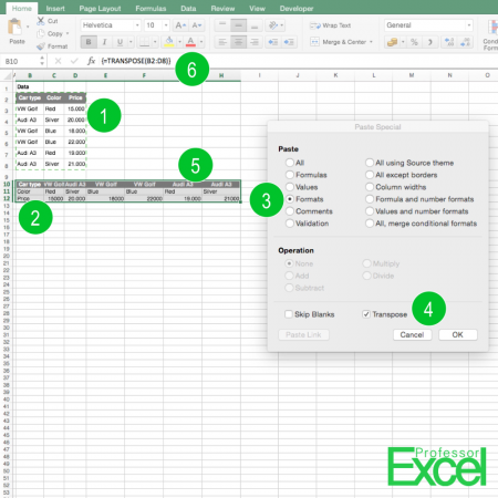
Follow these steps for setting a the array formula for pasting cells linked to their sources and transposing them (the numbers are corresponding with the picture on the right hand side):
- Copy the cells, which you want to transpose and link.
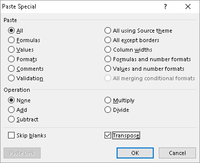
- Select the left top cell of the area you want to paste them to and open the paste special window by pressing Ctrl + Alt + v.
- Select “Formats”.
- Select “Transpose” and confirm with “OK”. Now, instead of values, just the original formatting is transposed. There are two reasons for this step: Getting to know the exact range for the transposed cells and at the same time already having the formats of the original cells.
- Select the whole paste area (or make sure it’s still selected after pasting the formats).
- Type this formula:
=TRANSPOSE('Original Range')and press Ctrl + Shift + Enter. If you only press Enter (without Ctrl + Shift) Excel won’t recognize your formula as an array formula. The curly brackets will be created automatically.
Method 3: Paste as link and transpose manually
Let’s take a look at the obvious method: Doing it manually. If your cell range is not too large it’s often the fastest solution. Of course, doing things manually is a source for possible errors.
- Copy your data and paste it with “Paste Special” by pressing Ctrl + Alt + v on the keyboard at the same time.
- There is a button “Paste Link” in the bottom left corner of the paste special window. Click on it and you’ll see, that Excel pastes the data as links.
- Now – and this is the annoying part – you have to drag and drop the cells to the their new places so that the rows and columns are exchanged.
Do you want to boost your productivity in Excel?
Get the Professor Excel ribbon!


Add more than 120 great features to Excel!
Method 4: Professor Excel Tools

As all the previous methods have some major disadvantages, pasting as link and transposing data was one of the first functions we’ve included in our Excel add-in:
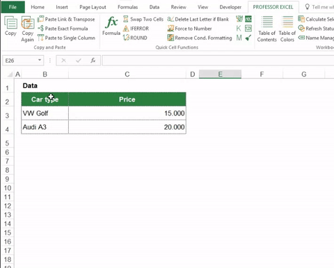
- Select your data and press copy on the left hand side of the Professor Excel ribbon.
- Select your target cell and press “Paste Link & Transpose” right next to the copy button.
This function works across workbook as long as source and target workbooks are open at the same time.


This function is included in our Excel Add-In ‘Professor Excel Tools’
(No sign-up, download starts directly)
More than 35,000 users can’t be wrong.