


You have received an Excel file with a PivotTable in it. Unfortunately, the file does not have the raw source data of the PivotTable. Or has it? Here are the steps for easily restoring the raw source data of the PivotTable.
Step 1: Check, if the source data is really not included
As the first step, make sure that the source data is really not included in your Excel file. If you are sure, proceed with step 2 below.
Why should you check this first? The reason is that seeing the source data has the advantage (compared to “restored” PivotTable data as we will see in Steps 2 and 3 below) that formulas, functions and formatting is intact.
How to check the source data of a PivotTable?

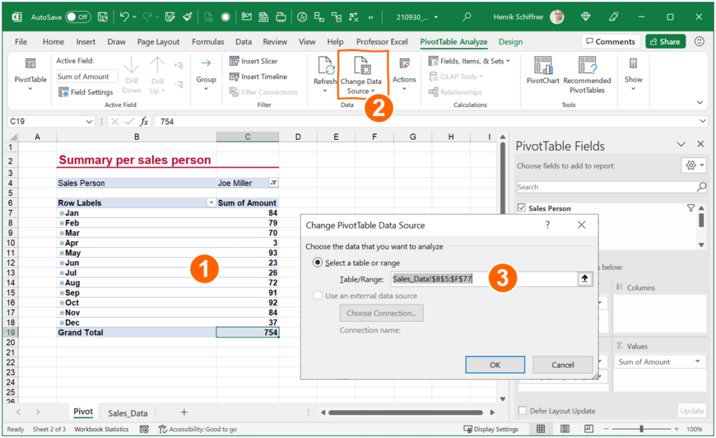
- Select a cell within your PivotTable.
- On the PivotTable Analyze ribbon, click on “Change Data Source”.
- If the Table/Range field refers to a source within your current file, navigate to it. It’s possible that the sheet is hidden or even very hidden – in this case, unhide it.
Step 2: Prepare the PivotTable
Let’s start with preparing the PivotTable so that we can restore all underlying data.
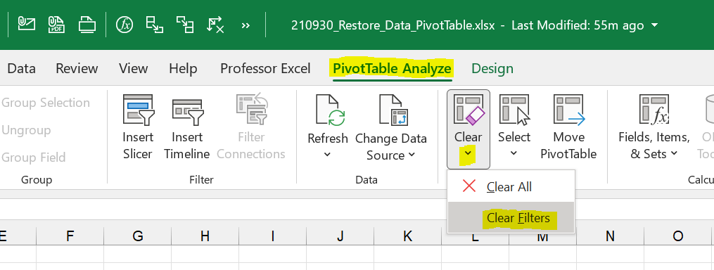
Step 2a) Remove all filters from the PivotTable
First, remove all filters. You can see all the filters in the PivotTable Fields list as highlighted below. You could also go directly to the PivotTable to remove the filters, but there is a chance that you could miss filters.
Go to the PivotTable Analyze ribbon, click on the small arrow under the “Clear” button and then on “Clear Filters”:

Step 2b) Add Grand Totals to the PivotTable
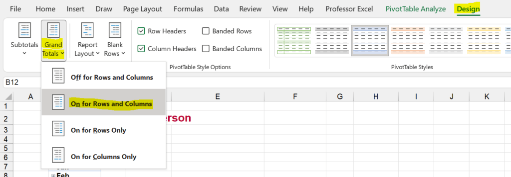
Next, show all Grand Totals.
- Click on any cell within the PivotTable.
- Go to the Design ribbon.
- Click on Grand Totals and then on “On for Rows and Columns”.

That’s it, we are done with the preparations! Let’s restore the data now.
Do you want to boost your productivity in Excel?
Get the Professor Excel ribbon!


Add more than 120 great features to Excel!
Step 3: Restore the source data of the PivotTable
Your PivotTable now has all the Filters cleared and Grand Totals. For restoring all the data, simply double-click on the cell with Grand Totals for both rows and columns.

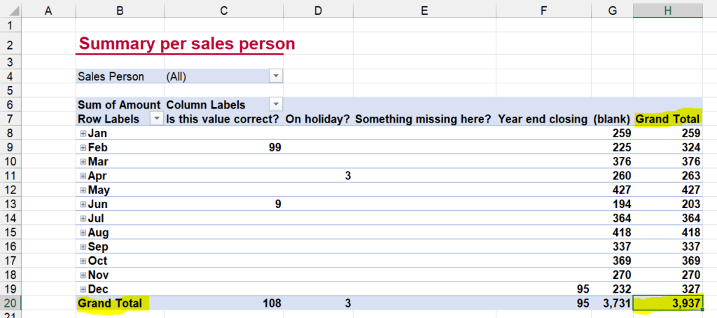
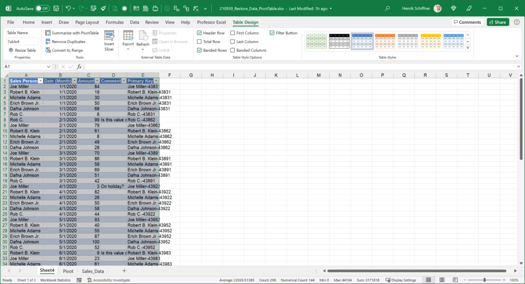
Excel now creates a new worksheet containing all data. It looks similar to this and is formatted as an Excel table.

Restrictions
PivotTable copy – plainly speaking – all the data into a cache. When you copy or move a PivotTable, the worksheet with the containing the data might not be available – but the PivotTable cache is. From this cache, we restore the data. There are, however, a few restrictions:

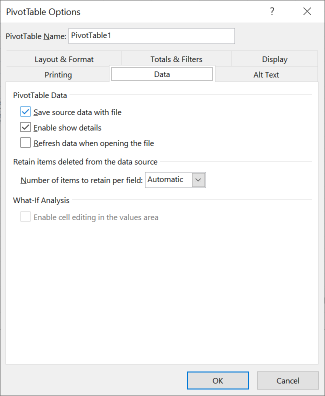
- It doesn’t work if the data is not saved with the PivotTable. Right-click on any cell in the PivotTable, then click on “PivotTable Options” and go to the Data tab as shown on the screenshot on the right. If the checkmark of “Save source data with file” is not set, you cannot restore the data.
- On the same Data tab in the PivotTable options: If the checkmark of “Enable show details” is missing, click on it in ordert to check it.
- It must be a real PivotTable. If you – for example – use the Break Links feature of Professor Excel Tools, the source data can not be restored.
- It usually also doesn’t work if the worksheet with the PivotTable on it is protected.
Image by Hans Braxmeier from Pixabay