


You have an Excel table and want to sum up all numbers in a column – but only, if one or more criteria are fulfilled. This is exactly, what the SUMIFS formula does: The formula adds up all numbers, when one or more than one criteria is fulfilled. The formula only exists since Excel 2007 and is especially useful, as it can regard several search criteria.
When to use the SUMIFS formula
The SUMIFS formula is very versatile and can be used in many cases.
- The basic case is to sum up values under one or more conditions.
- It is also very helpful in cases when you want to look up values, similar to VLOOKUP. But it can only be used for looking up numeric values (more on when to use VLOOKUP, SUMIFS or INDEX/MATCH).
- There are also some special applications as putting values into classes.
- Furthermore, it can be used horizontally. More on these cases later on.
With so many use cases, the SUMIFS formula is one of the most powerful formulas in Excel. So it’s worth spending some time learning how to use it.
How to use the SUMIFS formula

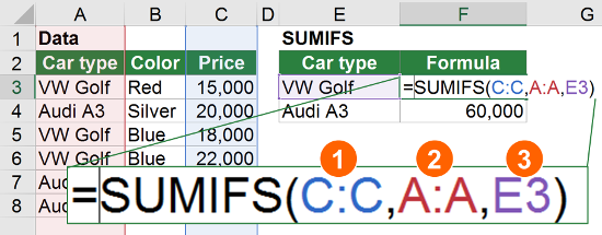
SUMIFS is very straightforward, although the formula can get quite long (the numbers are corresponding to the image on the right hand side):
- The column with the values you want to sum up.
- The column which your criteria is in.
- The lookup value (your criteria).
- Optional: Second criteria column.
- Optional: Second lookup value.
- …
In the example above, you sum up the prices of all VW Golf in cell F3.
Please note: SUMIFS is quite similar to SUMIF (without “s”). But SUMIF can only regard one criteria, whereas SUMIFS can match up to 127 criteria. So it is recommended using with SUMIFS, even if you only have one criterion.
Example with two criteria

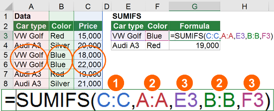
The first example above just had one criterion. As a next example, you got two search criteria. The image on the right-hand side shows the example with the following arguments in the SUMIFS formula:
- The first argument is always the range of values which should be summed up. Here, the values are located in column C.
- The first search array is column A. As you can see in the image, column A contains the car type.
- The third argument of the SUMIFS formula contains the first search criteria. It must match to the second argument above, in this case it refers to cell E3. As expected, cell E3 has the car type “VW Golf”.
- The second search array is column B.
- In column B, you search for the color. Cell F3 says “Blue”.
That means, you search for all blue VW Golf cars and sum up their prices. The encircled values in the table fullfil these criteria.
Special case 1: Sum up all values that are unequal to a search value
The default usage of SUMIFS is to sum up all values if some criteria are true. For example: Sum up all values from column D if there is “VW Golf” written in column B. Fortunately, the SUMIFS formula also works the other way around: Sum up all values if there is not written “VW Golf”. There are three different cases:
- A numeric value within the formula. Example: =SUMIFS(A:A,B:B,”<>”&2017)
- A text value within the formula. Example: =SUMIFS(A:A,B:B,”<>VW Golf”)
- A text value in another cell. Example: =SUMIFS(A:A,B:B,”<>”&D1)
Please note: <> stands for “unequal”. It (“<>”) must always be written in quotation marks like in the examples above.
Do you want to boost your productivity in Excel?
Get the Professor Excel ribbon!


Add more than 120 great features to Excel!
Special case 2: SUMIFS horizontally

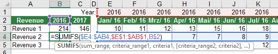
The SUMIFS formula works also horizontally. Instead of columns, you can define lookup rows and criteria rows. It works exactly the same as vertically. So let’s take a look at an example.
You got monthly data in the columns E to AB. For every month, there are 3 revenue values. You want to summarize them into years.
- First step: Insert a row for extracting the year. The formula in E1 would be =YEAR(E2). You use this row as the criteria range.
- Now you can set up the formula as shown in cell B2:
=SUMIFS($E3:$AB3,$E$1:$AB$1,B$2)
That means:
- You sum up the values in the range E3 to AB3.
- But you only sum them up, if in range E1 to AB1 is the value from cell B2.
In conclusion: You sum up the values in E3 to AB3, if in E1 to AB1 is 2014 (the value from B2). You could insert the $-signs so that if you copy the formula, the ranges won’t change.
Special case 3: Classify data with SUMIFS
Instead of a fixed criteria, you can also use “<” and “>”. So if you want to sum up all the values in column B with a search criteria in column A larger than 5, the formula would look like this:
=SUMIFS(B:B,A:A,”>5″)

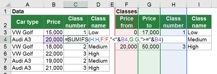
You can use this approach for classifying data. You got the following tables:
On the left hand side, there are two columns with cars and their prices. You will use these prices for classifying the cars into Low, Medium and High prices. How do you start?
- Prepare the classification table on the right hand side:
- It’s important, that each class has the lower class limits as well as the upper class limits. So cell F3 must have a value, although this class just means “less than 17,000”.
- As the SUMIFS formula can only return numeric values, you have to add a step in between. Instead of right away returning the class names Low, Medium, High, you return the values 1 to 3. This is done in column H.
- Eventually, you write the names of our classes into column I.
- Now you can go back to our original table on the left hand side. The formula in column C is:
=SUMIFS(H:H,F:F,”<“&B4,G:G,”>=”&B4)
That means:
- You sum up the values in column H. But as each criteria combination only appears once, it’s not really a sum but rather a lookup. You look in column H for the value to return.
- In column F, you search for the value smaller than the value in B4. You combine our criteria value with “<“&.
- In column G, you search for the value greater than or equal B4. So only if these two criteria are fulfilled, the value from column H will be returned.
3. As the returned value is only a number and you want to get the corresponding name Low, Medium or High, you use a simple VLOOKUP in column D (more information about the VLOOKUP formula). The formula in D4 is:
=VLOOKUP(C4,H:I,2,FALSE)
Step 2 and 3 can be merged into one step. But the structure keeps clearer if they are still separated into 2 steps.
Special case 4: Wildcard criteria
If you don’t want to search for exact matches within your criteria range, you can use wildcard characters. There are two wildcard characters:
Asterisk (*):
An asterisk matches any sequence of characters. For example, you want to search for any string starting with ‘prof’. Then the formula could look like this:
=SUMIFS(H:H,F:F,”prof*”)
It doesn’t matter, how many characters or which characters follow after ‘prof’. Excel will sum up all values in column H for which the value in column F starts with ‘prof’.
Question mark (?):
The question mark indicates, that one character could vary. Let’s take a look at an example:
=SUMIFS(H:H,F:F,”abc?”)
That means, that you search in column F for a 4 character word, starting with abc. The last character after ‘abc’ can vary
What if you want to search for a question mark or asterisk?
There are some cases in which you might want to search for exactly * or ? . You can use this trick: add the tilde ‘~’ in front of the question mark or asterisk. That way, that wildcard function of the character will be disabled.
Solving errors with the SUMIFS formula
- You got a wrong result, for example the returning sum is not as expected? Make sure that all criteria ranges have the same size, for instance, column A1:A5 and B1:B5
- #NUM! errors: It’s possible that you sum up too large values or that at least your result exceeds the maximum possible number in Excel.
- You get a 0 (zero) returned, although there should be another value? Most probably, the search criteria don’t match. When VLOOKUP returns a #N/A error, SUMIFS just returns 0.
- For other errors, please check out the error helper. Select your error message in the upper box and SUMIFS in the lower one. Press ‘Solve error’ to receive more information about the error and in combination with SUMIFS.
Download all examples
Please feel free to download all examples above in one Excel file.
- File name: Example_SUMIFS.xlsx
- Link: Click here (opens in new tab)
- Size: 21 KB