


Microsoft quietly replaced the comfortable Text Import Wizard from Excel and replaced it with the “Get & Transform” tools. The “Get & Transform” tools offer a lot of options and are very powerful. Unfortunately, they are quite complicated to use. Here is what you should now.
In a hurry? Click on “File” –> “Options” –> “Data” and set the corresponding checkmarks for reactivating the “Text Import Wizard” in Excel. Start the text import by clicking on “Data” –>”Get Data” –> “Legacy Wizards” –> “From Text (Legacy)”.
Introduction
In Excel 365 (only) 2016 (since version 1704) the “Text Import Wizard” was removed. It was replaced by the powerful “Get & Transform” tools. The “Get & Transform” tools also provide a function to import text and CSV files into Excel.
You have the following two options:
- Luckily, the comfortably “Text Import Wizard” still exists. You can re-activate and use it for importing text and csv files into Excel.
- Use the import function of the “Get & Transform” tools.
Restore the “Text Import Wizard”

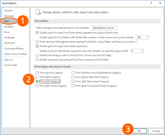
The good news: You can easily restore the “Text Import Wizard”. Unfortunately, the option for re-activating them is hidden.
Follow these steps:
- Click on File and then on “Options”. Go to “Data” on the left-hand side.
- In the lower section of the window you can select the wizard you’d like to restore. For only importing text- or csv-files, select “From Text (Legacy)”. Feel free to also activate the corresponding wizard for importing Access files, files from web, from SQL servers and so on.
- Confirm with OK.

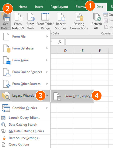
Now, you can find the so-called “Legacy Wizards” in the “Get Data” drop-down menu. In order to use them, follow these steps:
- Go to the “Data” ribbon.
- Click on “Get Data” on the left-hand side.
- Next, go to “Legacy Wizards”.
- Click on “From Text (Legacy)”.
How to use the “Text Import Wizard”

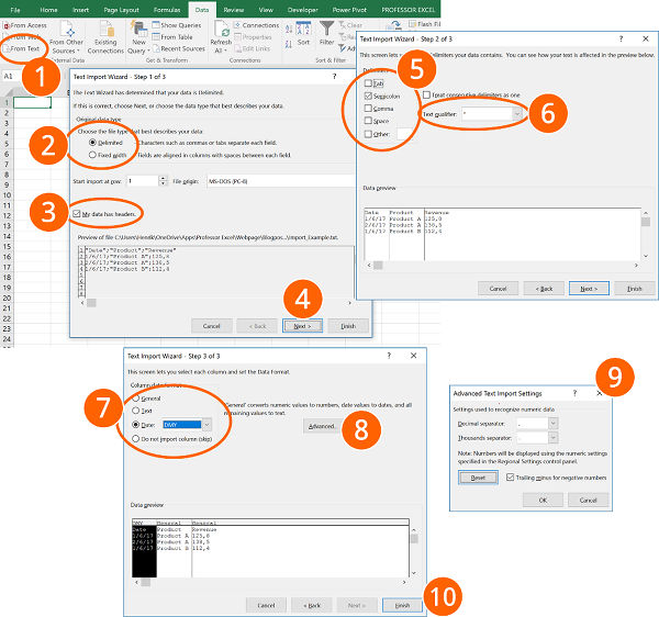
The steps for using the “Text Import Wizard” in Excel are shown in the screenshots.
- Go to the “Data” ribbon and click on “From Text”. If you have a recent Excel version and there is no button called “From Text” (but instead “From Text/CSV”), click on “Get Data”, then on “Legacy Wizards” and then on “From Text (Legacy)”. Please refer to the paragraph above if this option is missing.
- Select how you want to define the columns: Either with a character as a separator or with a fixed width.
- If the first row contains headers, check the corresponding box.
- Continue with “Next >”.
- Select the delimiter. This is the character dividing the data into columns, for example “Tab”, “Semicolon” or “Comma”.
- Usually text fields use quotation marks marking the beginning and end of a text field.
- For each column, you can choose the data format. For dates, you could define the order of days, months and years.
- Click on “Advanced”…
- …for defining decimals and thousands separators.
- Finalize the import by clicking on “Finish”.
Import text and csv files with the “Get & Transform” tools


Importing text files in Excel with the “Get & Transform” tools requires many steps. Please refer to the numbers on the screenshots:
- Click on “From Text/CSV” on the “Data” ribbon in order to start the import process.
- Choose the delimiter (e.g. semi-colon, comma etc.). Here you can also switch to “Fixed Width”. If you want to separate your import data with the “Fixed Width” option, you have to type the numbers of characters, after which you want to data to be divided.
- For further options (e.g. switching thousands- and decimal separators) click on “Edit”.
- If you data is not represented correctly, delete the automatically created step “Changed Type”.
- Change the date format: Right-click on a column that contains a date. Alternatively click on the small “ABC” symbol in the top left corner of the column heading.
- Move the mouse to “Change Type”.
- Click on “Using Locale…”.
- Select “Date”.
- Select the locale format for dates. In this example, the German date format is used.
- Confirm with OK. Repeat the steps 5 to 10 for each date column.
Recommendation: Select several date columns at the same time by pressing and holding the Ctrl key while selecting the columns. - Change the decimal and thousand separators: Right-click again on a column with decimal numbers.
- Move the mouse to “Change Type”.
- Click on “Using Local…”.
- Choose “Decimal Number”.
- Select the local number format. Please refer to this article for a list of local number formats.
- Confirm with “OK”.
- Last step: Insert the data into a worksheet. In order to achieve this, click on “Close & Load” in the top-left corner.