Pivotable: How to Prepare Data for Creating Pivot Tables in Excel

Pivot Tables are one of the most helpful features in Excel. With Pivot Tables, you can easily evaluate data. Per drag-and-drop you arrange analysis layouts. Within seconds, you’ll see your results – without using any formulas. Usually the first obstacle comes up, when you try to create a Pivot Table. There are some rules to regard in order to create Pivot Tables and your data needs a certain structure. In this article we explore how to make your data ‘pivotable’.

In this article: 

• Starting point: We got a “normal” Excel table.
• Goal: We want to create a Pivot Table from it.
• Topic: With this example, you learn how to structure the data and the requirements for creating Pivot Tables. You learn how to make a normal Excel table “pivotable”.
• Comments: The example is typical. The solution won’t fit to every other table, but the approach should be applicable.

Steps for creating Pivot Tables

In our previous article you’ve already learned about the purpose of Pivot Tables. We’ve also talked about the steps for setting up a Pivot Table in detail. To insert a Pivot Table in Excel, please follow these steps:

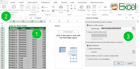
1. Select the input data.
2. Click on ‘Pivot Table’ on the ‘Insert’ ribbon.
3. Follow the steps on the screen. After confirming with OK you can drag-and-drop the fields for arranging the Pivot Table.

Please refer to the previous article for more help on the steps. For now, we want to concentrate on the requirements of your data and how to make your data ‘pivotable’.

Requirements for Pivot Tables

The data for your Pivot Tables must meet the following requirements:

1. The most important criteria: Each column must have a title. The title is always the top row of your data. Blanks/ empty cells as column headings are not allowed.
2. In earlier versions of Excel, each column heading could only appear once. Therefore, each column heading had to be unique. Newer version add a number in the end if a title is used several times. In order to avoid confusion, we recommend using unique column titles for each column.
3. Your data should have a ‘database’ structure: Each column should have one criteria or value. If you use the ‘table format’ in Excel already, you shouldn’t have any problems.

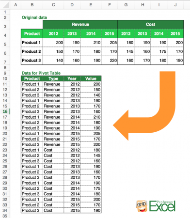
Please take a look at the image on the right. The upper table is not formatted well for creating a Pivot Table. But the lower one is ‘pivotable’. It has 4 columns and each column has a single purpose or data item.

Example: Make an existing table ‘pivotable’ so that you can create a Pivot Table from it

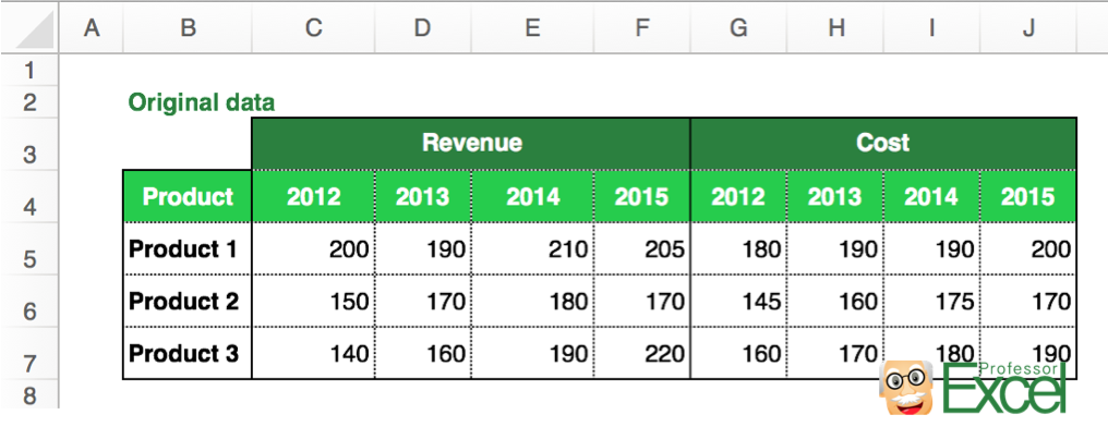
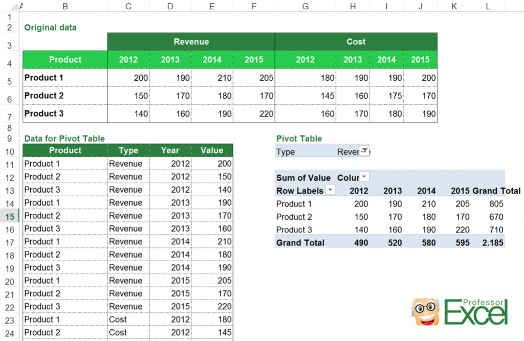
Let’s assume you have the table above and you want to create a Pivot Table with it. Therefore, you have to change the structure.

Each row contains the values of one product. The columns C to F show the revenue per year and the column G to J the corresponding costs.

That means, you got 4 different types of data: The product name/ number, the type (revenue, costs), the year and the values.

In order to create a Pivot Table, you need a structure as shown on the right hand side. Each column contains one data type. As you have 4 different data fields (product, type (revenue or cost), year and the values) you need 4 columns, one for each data type.

So let’s start filling the columns. This requires some manual steps as well as some formulas.

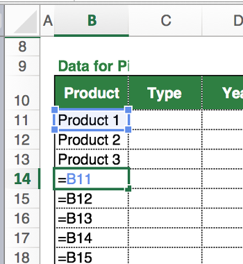
• Product: You only have 3 products, so it’s not too difficult preparing the first 3 rows. Just copy and paste the cell B5 to B7 from the original table.
  But you need the rows several times: In total, you need each product for every year (2012, 2013, 2014, 2015) two times (revenue and costs). Because you got 3 products, you need 24 (2 types x 4 years x 3 products) rows plus the header row.
  You have two options: repeat this step 8 times or think of a shortcut. In our small example manually repeating this copy-and-paste procedure is possible. But what if you got more than 3 years or more than 2 types of data?
  So, the easiest way is using this formula in cell B14: =B11 . This formula you can easily copy down and the 3 products will keep on repeating.

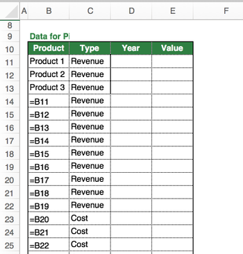
• Type: With the column ‘Type’ you classify if the value is revenue or cost. So you need 12 rows saying ‘Revenue’ and 12 rows saying ‘Costs.
  Why 12 rows? You got 3 products, and each products needs 4 rows for the years 2012, 2013, 2014 and 2015. So that makes 12 rows (3 products x 4 years).
  Probably the fastest way: Write “Revenue” in cell C11 and copy it down.
  Do the same with “Costs”, starting in row 23 (as you start in row 11 + 11 rows of revenues) and copy it down to the last row as well.

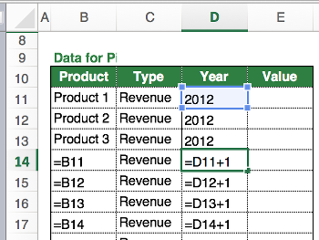
• Year: The first 3 rows should start with year 2012. The following 3 rows should say 2013 and so on. Therefore we write 2012 into the cells D11 to D13.
  In D14 we link to D11 but add 1. Copy and paste this formula down until the end of the revenue block. Then repeat the same for the cost (or copy the cells above).

• Value: Now the actual values are still missing. For the values you got two options: use a formula or an Excel add-in (well, besides copying each value manually):
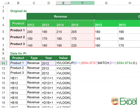
  • Method 1 – Formula: For each combination of product, type and year you need to get the correct value from the table above. Therefore you can use a two-dimensional lookup as shown on the picture on the right hand side.
    The formula is basically a VLOOKUP, searching for the product (here: ‘Product 1’ in cell B11) in the column B (given by the range $B$4:$F$7).
    Instead of using a fixed value for the return column, you search for the current year with the MATCH formula in the original cell range.
    The last 0 indicates, that we are searching for the exact match.
    The complete formula for revenues:  =VLOOKUP(B11,$B$4:$F$7,MATCH(D11,$B$4:$F$4,0),FALSE)
    Adapt the formula for the costs. The underlying structure is the same: =VLOOKUP(B23,$B$4:$J$7,MATCH(D23,$G$4:$J$4,0)+5,FALSE)  The idea is to change the return range to the right hand side.
    Copy these two formulas down for revenues and costs.

Method 2 – Add-in: Because the formulas are quite complicated, we’ve integrated a function in our Excel add-in ‘Professor Excel Tools’. It copies all values into one column underneath each other. Follow these steps:

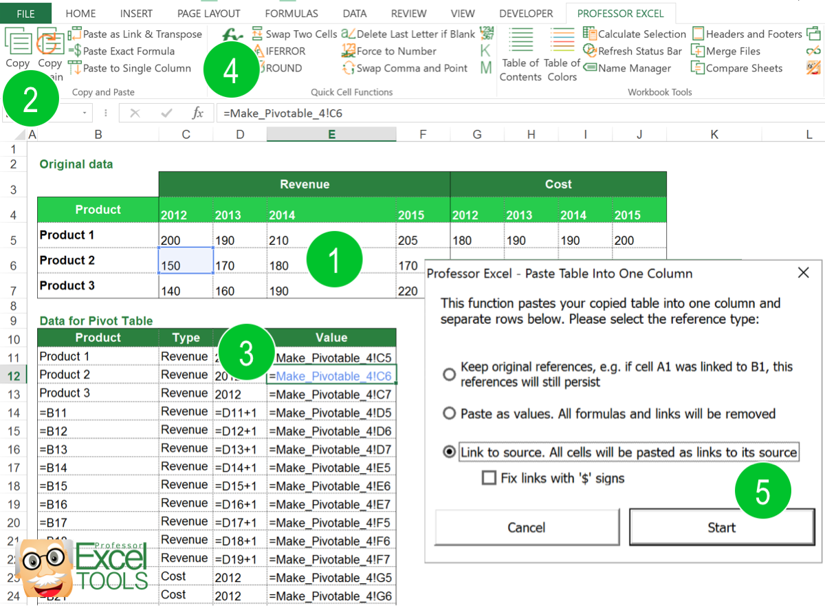
1. Select the source data.
2. Press copy on the ‘Professor Excel’ ribbon.
3. Select the cell, in which you want to start pasting the data (in your case E11).
4. Click on ‘Paste to Single Column’ on the ‘Professor Excel’ ribbon.
5. Select your desired option. Our preferred pasting option is usually ‘Link to source’ because any changes of the original values will be regarded. Confirm by clicking on start.

That’s it. Now you can insert a Pivot Table. The final result should look similar to the image on the right hand side.