


The queen of lookups in Excel: The 3 way- or 3D lookup. Imagine this scenario: You have several Excel tables, each has rows and columns. Depending on your input values, you want to get the data from a specific cell from the right table, row and column. Such lookups are called 3D lookups or 3 way lookups. In this article we explore 6 methods of how to conduct 3D lookups in Excel.
What is a 3D lookup?
The 3D lookups are advanced lookups in Excel. The basics are the same like any lookup, e.g. VLOOKUP: You search for a specific value. But the VLOOKUP formula is (in it’s basic version) just 1-dimensional (you only search within rows). 3D lookups don’t only search in rows, but also in columns (well, until here you only got 2 dimensions). The third dimension is added by the search table itself: 3D lookups search in rows, columns and tables at the same time.
Preparations: The basic formulas for 3D lookups
The following methods are based on 4 basic formulas in Excel. Each formula we’ve described before, so please refer to these articles if you need assistance:
Also, you should get yourself familiar with the 2D lookup, as 3D lookups build up on this. Furthermore – but not necessary – you could take a look at this article: It describes, when to use which lookup formula.
Please feel free to download the example file here. It contains all the examples described in this article.
Overview of all example methods
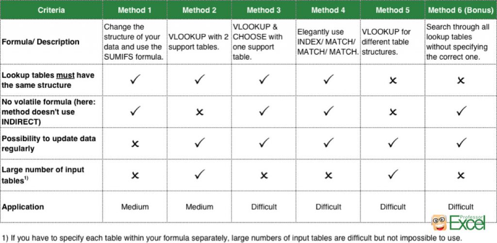
As this article is quite long, we provide you an overview of the 6 methods. That way, you can scroll directly to your best method.

6 methods of 3D lookups for equal table structures

Before we jump in with the four methods for 3D lookups, let’s take a look at our underlying example first.
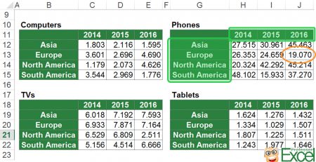
You got the four tables as shown in the image on the right hand side.
The task: Depending on the type, region and year you want to get a specific value. For example, you want to know the number of phones sold in 2016 in Europe.
Please note: There are countless approaches and methods. In this article you learn 6 different versions. You can of course – based on your data – change or combine these methods.
Method 1: “Cheating” by changing the structure of your data
First step: Change the structure of your data

The first method is actually not really a 3D lookup but oftentimes the best and fastest solution. You change the structure of your data so that you can conduct a “normal” 2D lookup. In our example it’s easily possible as all the four tables got the same structure with the same rows and columns.
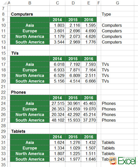
Start by copying the tables underneath each other. Then you add one column, containing the type. As you can see in column G, it always says “Computers” and “Phones” and so on. This column will be part of the lookup.
Now you use the SUMIFS formula (if you are not sure if the SUMIFS formula is possible in your case, please refer to this article).
The solution looks something like this:

Second step: Set up the SUMIFS formula
The SUMIFS formula has got two crucial parts in this example:
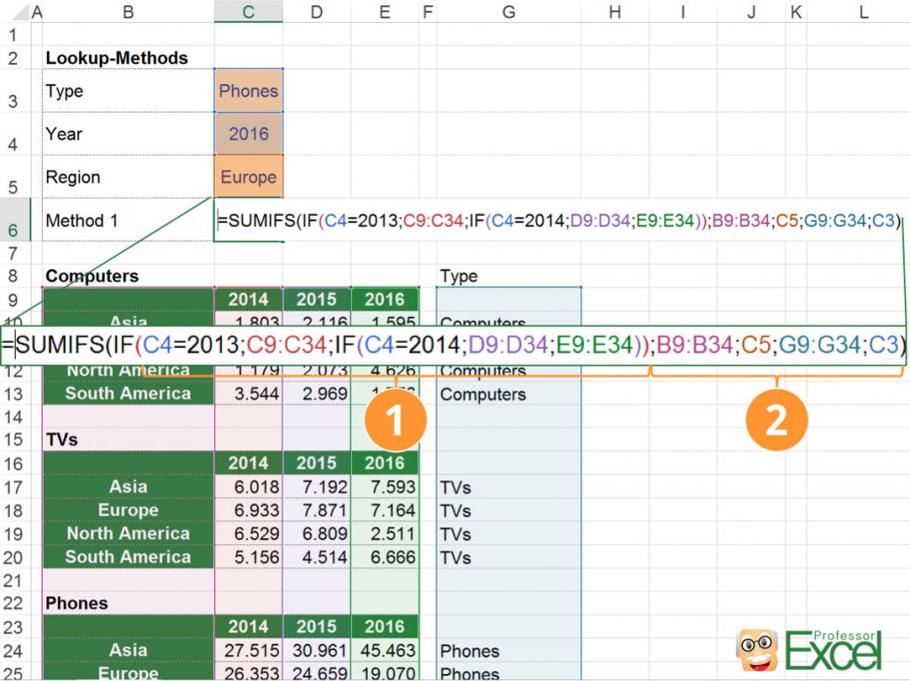
- The return column which you want to get the value from. In this example the return column depends on the year you select. If it’s 2014, you have to get the value from column C. For the year 2015 you get the return value from column D and otherwise (e.g. 2016) from column E.
In order to keep the formula simple, we decided to use the IF formula. Of course, you can also use other methods, e.g. VLOOKUP in combination with INDIRECT. But that way you would need one more support table. - The second part of the SUMIFS formula contains all the other criteria. In this case it’s the country in column B and the type in column G.
The complete formula is:
=SUMIFS(IF(C4=2013,C9:C34,IF(C4=2014,D9:D34,E9:E34)),B9:B34,C5,G9:G34,C3)You should use this method if
- all your data is in the same format,
- you won’t update your data regularly,
- you are looking for a simple solution.
Method 2: The easy way with VLOOKUP & INDIRECT
First step: Set up support tables

The next method of 3D lookups is based on the VLOOKUP formula. Unfortunately, the VLOOKUP formula is by default not made for advanced lookups. That’s why we start by creating two support tables:
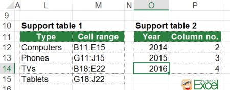
- Support table 1 contains the ranges of the tables, e.g. the data for computers is located in the cell range B11 to E11. It’s important that you include the lookup column (here: the countries). The VLOOKUP will search in this first column.
- The second support table contains the return column, counting from the search column. For example, you search for computers in column B, then the value for the year 2014 is located in the second column counting from column B. As all your tables have the same structure, the return column are always the same.

Second step: Create the VLOOKUP formula
Now you can start setting up the VLOOKUP (if you need more assistance with the VLOOKUP formula, please refer to this article). The idea is, that you use a VLOOKUP searching for the country. But instead of having fixed search tables and return columns, you make them variables too.
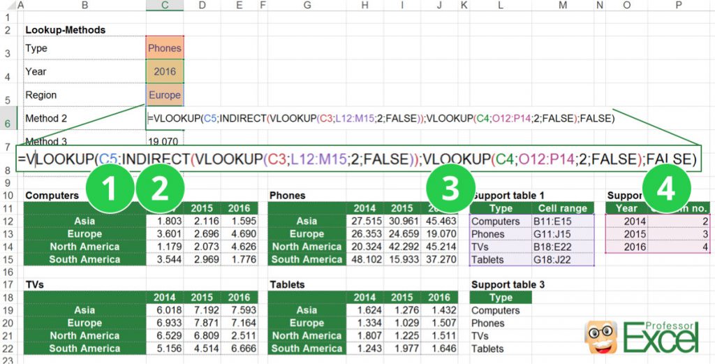
- That means, the first part of your VLOOKUP formula is the country (given in cell C5).
- Now it slowly gets tricky: The search table changes depending on the type. E.g. if you search for computers, you have to search in the cell range B11 to E15. To achieve this, you get the range from your first support table with another VLOOKUP. You wrap the VLOOKUP formula with INDIRECT so that the return value from the VLOOKUP formula is a cell reference and not just text.
- The return column is variable, too. It changes depending on the year you select. Therefore, you use another VLOOKUP in your second support table.
- The fourth part is – as usually – just “FALSE”.
The complete formula:
=VLOOKUP(C5,INDIRECT(VLOOKUP(C3,L12:M15,2,FALSE)),VLOOKUP(C4,O12:P14,2,FALSE),FALSE)You should use this method if
- your data is in the same format,
- you are comfortable with the VLOOKUP formula,
- you are looking for a simple solution.
Please note: If your data is located on different worksheets, just add the sheet name to the first support table. Instead of B11:E15 you would write ‘Sheet 1’!B11:E15.
Do you want to boost your productivity in Excel?
Get the Professor Excel ribbon!


Add more than 120 great features to Excel!
Method 3: The inconvenient way (VLOOKUP, CHOOSE and MATCH)
First step: Set up a support table

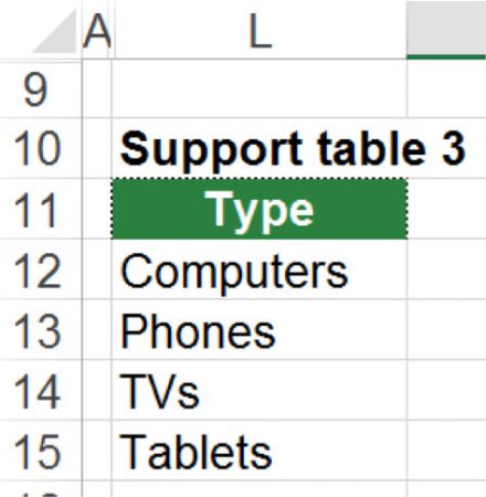
The third method of 3D lookups is similar to the second method: It’s based on the VLOOKUP formula. But in this example, you only need one support table. This time, the support table only contains all the types, e.g. computers, phones. You’ll use this with the MATCH formula.
Now you can start putting the VLOOKUP formula together. The difference to the second method: You don’t use the INDIRECT method for switching the lookup table. Instead you use the CHOOSE formula. Furthermore, you take a shortcut for the lookup column with the MATCH formula instead of another support table.

Second step: Create the VLOOKUP formula
The four parts of the VLOOKUP formula:
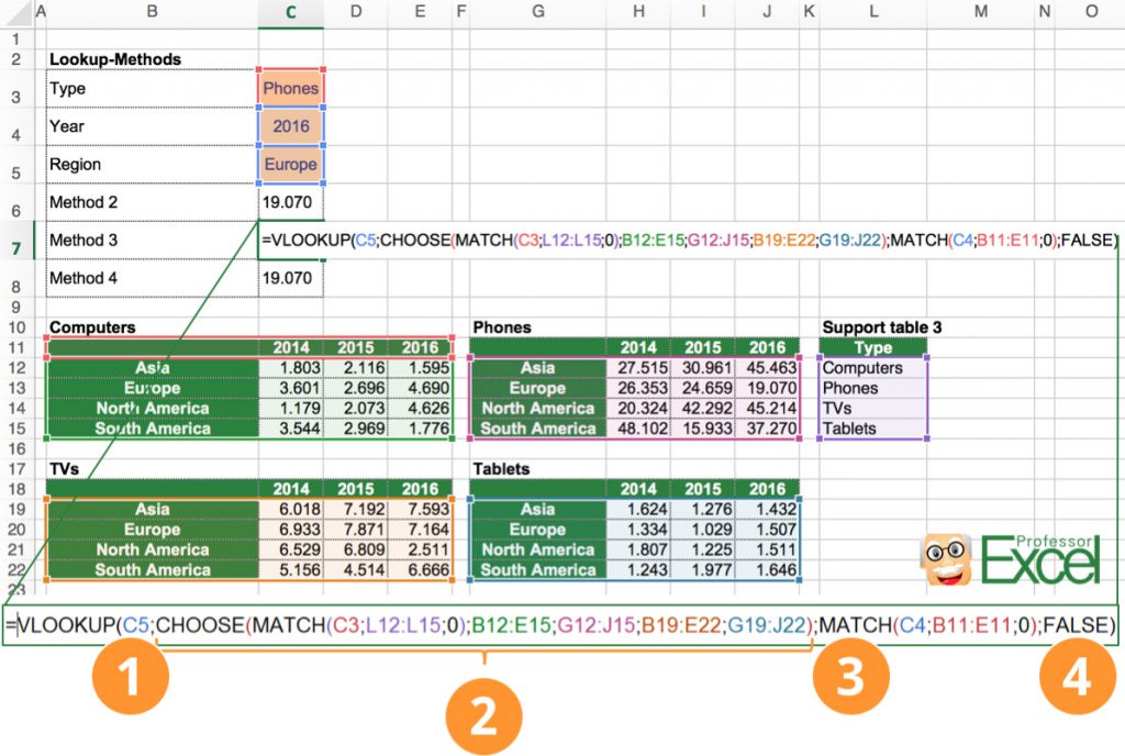
- You look for the country, given in cell C5.
- The search area depends on the type you’ve selected. In this case, you use the CHOOSE formula. The structure is simple: you provide the number of the table you want to use as well as all the table references. Depending on the number – let’s say 2 – the CHOOSE formula returns the second cell range you’ve provided.
With the MATCH formula, you find out the number of the table you need. Therefore you use the support table. It has the correct order of types. So if you search for “Phones”, the MATCH formula returns “2”. This number 2 refers to the second cell range you’ve given. In your case it’s G12:J15. - As the structure of all tables are equal, you can just use one table for identifying the return column. For that, you use the MATCH formula again.
- As usual, the last part of VLOOKUP is just “FALSE”.
What if your tables don’t have the same structure? E.g. one table misses the column 2014? In such case, you have to modify the third part of the formula. The MATCH formula must get the return column from the correct table. You could either use another CHOOSE formula within the second part of the MATCH formula or the INDIRECT formula, similar to the description of method 2.
You should use this method if
- your data is in the same format (if not, you could extend the third part is said before),
- you are comfortable with the VLOOKUP formula,
- you want to avoid the volatile INDIRECT formula.
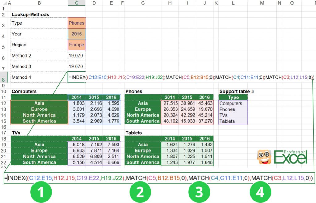
Method 4: The elegant way for 3D lookups (INDEX & MATCH & MATCH & MATCH)
First step: Set up a simple support table
The 4th method is probably the most elegant approach: A combination of INDEX and 3 MATCH formulas. Again, you need one support table (it’s the same of method 3). It only contains a list of the input tables, in your case “Computers”, “Phones” and so on.
Having this, we can start setting up the INDEX formula.

Second step: Create the INDEX formula
- The first part of the INDEX formula contains references to all four input tables. The ranges, e.g. C12:E15, H12:J15, are divided by commas (sorry, the screenshot above shows semi-colons, which is due to the German number system). This section of the formula is embraced by brackets.
- The 2nd part determines the row of the return value with a MATCH formula. As all four tables have an equal structure, you can just link to one of them. In this area, you search for the country.
- The 3rd part of the formula returns the number of column. Again, because the tables are exactly the same, you can just link to one of the and search for the year. The MATCH formula returns the number of column.
- For the last part you determine which table you want to get the value returned from. Therefore you search within your support table for the country with the MATCH formula. The MATCH formula returns the correct number.
This number must correspond to the first part of the formula: Let’s say you want to get the value of phones. In your support table you search for phones with the MATCH formula. The return value is 2, as phones are the second entry of the support table. Now Excel takes the second range from the first part of the INDEX formula (from the references to the 4 tables).
You should use this method if
- your data is in the same format,
- you are looking for an elegant option,
- you don’t mind if most other users won’t understand your solution and
- you want to avoid the volatile INDIRECT formula.
Method 5: 3D lookups if the tables don’t have the same structure…

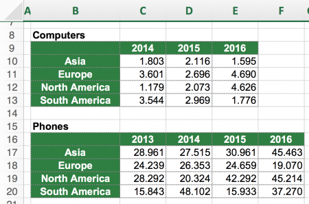
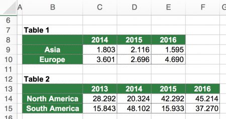
Unfortunately, in many cases the input tables don’t have the same structure. That’s why we take a look at another example of 3D lookups with different input tables. In order to keep it simple, we just go with 2 different input tables as shown in the table on the right hand side.
The difference: The lower table on the right hand side has a new column C with the year 2013. In this case we modify the 2nd method from above.
First step: Setting up the support tables

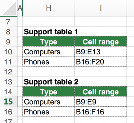
The basic formula is still a VLOOKUP but you use two support tables. These support tables are quite similar and we use them with INDIRECT formulas, so that they contain ranges.
The first support table contains the complete ranges, in which you want to search either for “Computers” or “Phones”. It’s important, that the leftmost column (here: B) is included as we search within this column.
The second support table has the ranges of the headlines of each table. In these headlines we will search for the return column.
Second step: Create the VLOOKUP formula

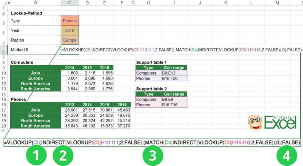
The VLOOKUP formula has always four parts:
- You again search for the region. That was the simple part of the formula 😉
- With the INDIRECT formula you determine the search range. Therefore you search with a short VLOOKUP formula within the 1st support table. This is either the range of the first table (“Computers”) or the second one (“Phones”).
- Now comes the tricky part: You have to find out, in which column your return value is located. This is different depending on each table: If you search for computers in 2016 the return column is E whereas for phones it’s column F.
You do this with the MATCH/ INDIRECT combination. MATCH searches for 2016 and with INDIRECT you determine the search range. - The last part is “FALSE” as usual.
Bonus: Search in several lists for one item

Let’s take a look at one more version of 3D lookups: Search through several tables for a specific item. That means, you don’t specify, in which table your data is located. You rather let Excel go through all of them until found.
The example is quite simple: You got the 2 tables as shown on the right hand side. You search for a specific country and year combination.
The solution is actually quite simple: Do you remember the (comparatively easy) 2D lookup? Please refer to this article – we will use the 4th method from that article without going further into detail.
The trick: Use two 2D lookups, one for each table. Then you combine them with the IFNA formula. The complete formula looks like this:
=IFNA(INDEX(B8:E10,MATCH(C4,B8:B10,0),MATCH(C3,B8:E8,0)),INDEX(B13:F15,MATCH(C4,B13:B15,0),MATCH(C3,B13:F13,0)))Conclusion
You’ve learned 6 different methods in this article. All methods have advantages and disadvantages. Now it’s your task to pick the most suitable one and taylor it to your needs. The methods usually require some practice and trial-and-error. So if they don’t work instantly, please be patient and check for the errors. With time going by you will feel more comfortable.
Please also feel free to download the example file here. It contains all the examples described in this article.