


You’ve probably heard of the VLOOKUP formula in Excel, haven’t you? The VLOOKUP formula searches for a value in a column. Once found it returns another value from the same row. A combination of INDEX and MATCH serves the same purpose. It works slightly different and has therefore some advantages and disadvantages towards VLOOKUP.
First things first:
- Before we start with the VLOOKUP: Do you know XLOOKUP? It’s new in Excel and has some advantages towards INDEX/MATCH (and can do mostly the same as INDEX/MATCH but more straight-forward).
- When we say VLOOKUP in this article, we also refer to the HLOOKUP formula in Excel. It works the same way only with horizontal rows instead of vertical columns. This also applies for the INDEX and MATCH formula combination because it works the same way horizontally and vertically.
The INDEX formula
As INDEX and MATCH are two separate formulas, we take a look at them separately before putting them together.
The INDEX formula returns the n-th value from an array of cells.
Let’s say we got a range of 4 cells, for example D3:D6 (blue range in the picture above). We want to know the value of cell D5. As D5 is the 3rd value in this range, we type the following formula:
=INDEX(D3:D6;3)
The first part (number one on the picture), defines the array of cells which we want to get the return value from. The second part of the formula says, that we want to get the value of the third cell in this range.
The MATCH formula
With MATCH, you can search for a value within a range of cells. Once found, MATCH returns the location of the first occurrence.
An example: We got a cell range B3 to B6 with car brands (the red cell area in the picture above). We want to search for the brand “BMW” within this cell range. The result should be the number of the cell. Counting starts with the first cell of the range.
=MATCH("BMW",B3:B6,0)
So we search for “BMW” (first part of the formula, number 2 in the picture above), within the range B3 to B6 (second part of the formula, number 3 in the picture above). The third and last part of the formula is a little bit tricky:
- If you search for an exact value, just type 0 (zero).
- If you want to find the largest value that is less than or equal to the lookup value, type 1 or omit it. Please note, that the values most be sorted in ascending order. If not, you’ll get a #N/A error message.
- If you want to find the smallest value that is greater than or equal to the lookup value, type -1. In this case, the values must be sorted in descending order. If not, you’ll get a #N/A error message.
In our case we search for the exact name “BMW” so that we have to fill in 0 as the last part of the formula.
The combination of INDEX and MATCH

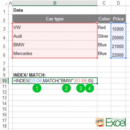
We now know how to use INDEX and MATCH separately so that we can combine them. In our example, we search for BMW in the first column (column B) and want to get it’s price from column D.
The formula has 4 relevant parts (the numbers are corresponding to the picture above):
- The first part refers to the cells containing the value that we want to get returned. In our case it’s the price.
- With the MATCH formula we will get the location of the first cell, that says “BMW”. The first part of the MATCH formula is the keyword we search for.
- The second part of the MATCH formula contains the range of cells, we search “BMW” within.
- We have to determine that we want to find the exact term “BMW” by adding “0” as the fourth part of the formula.
The complete formula looks like this:
=INDEX(D3:D6,MATCH("BMW",B3:B6,0))
Do you want to boost your productivity in Excel?
Get the Professor Excel ribbon!


Add more than 120 great features to Excel!
Advantages and disadvantages of INDEX and MATCH towards VLOOKUP
A combination of the two formulas INDEX and MATCH has some advantages and disadvantages towards VLOOKUP:
Advantages
- The INDEX and MATCH combination returns the value from any column. VLOOKUP on the other hand only returns a value on the right hand side of the search column.
- INDEX/MATCH also usually more stable, because the return column stays the same if you insert more columns in between.
- The INDEX and MATCH combination needs slightly less processing performance of your computer.
Disadvantages
- The main disadvantage of INDEX and MATCH is that it’s not well known. Therefore other people working on your workbook might not immediately understand it.
- Applying the INDEX and MATCH combination is comparatively difficult. There are some typical sources of errors: For example not having the same ranges or omitting the (often) necessary 0 in the last part of the MATCH formula.
If you want to know more about when to use VLOOKUP, SUMIFS or INDEX and MATCH, please have a look at this article.
Take it one step further: 2 way lookups with INDEX – MATCH – MATCH

Above you’ve learned the simple version of the INDEX formula in Excel. But there is an advanced way to use it too: You can not only provide one dimension for a lookup, but also a second one. That way, you can create a 2 way- or 2D lookup.
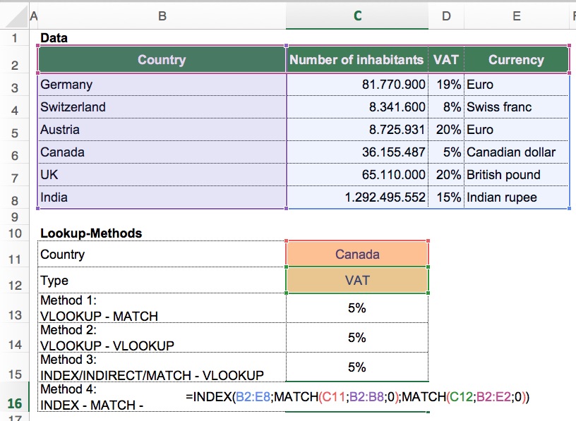
Instead of just a simple INDEX/MATCH combination, you can add one more dimension with the second MATCH. The formula looks like this:
=INDEX(B2:E8,MATCH(C11,B2:B8,0),MATCH(C12,B2:E2,0))
The INDEX formula has 3 parts here: The complete cell range (B2 to E8) and two MATCH formulas.
- The return cell range stretches over the hole table. In our case that’s B2 to E8.
- The first MATCH searches within the range B2 to B8 for the country.
- The second MATCH looks for the type in the cell range B2 to E3 (the headline).
Both MATCH formulas return the number of the cell in with the search term the first time comes up.
Do you want to know more about the 2D lookup in Excel? Please refer to this article.