


It seems as if Microsoft has listened to many complaints of Excel users and introduced a new formula: XLOOKUP. It’s supposed to improve all the disadvantages of the “traditional” lookup functions VLOOKUP, INDEX/MATCH and SUMIFS. This article describes in what case and how to use it. Please feel also free to download all example in an Excel workbook at the end of this article.
The XLOOKUP function is special in a way that it is very simple in it’s basic form. Just three arguments that are quite straight-forward. At the same time, it has very advanced capabilities. That’s why I’ve decided to split this article: The basic application, just using the first three arguments and advanced functions.
Overview of the big XLOOKUP series
- Part 1: Basics of XLOOKUP (this article)
- Part 2: Advanced XLOOKUP – “If not found”, “Wildcard” and “Classification”
- Part 3: 2D-XLOOKUPs
- Part 4: Let’s talk about performance of XLOOKUP
- Part 5: Convert XLOOKUP to VLOOKUP
XLOOKUP: Introduction
Microsoft describes XLOOKUP as follows:
“Searches a range or an array for a match and returns the corresponding item from a second range or array. By default, an exact match is used”
Well, this sounds quite dry. To put it more exciting words: It can do everything VLOOKUP (and mostly also INDEX/MATCH) can do. But much more! I’m sure, this will be the future of lookups in Excel. Before we start, let me already summarize, why I think that XLOOKUP is a great replacement for VLOOKUP (and HLOOKUP, for that matter):
- The sequence of columns (or rows) doesn’t matter any longer. So, the search column doesn’t have to be the leftmost column in your table.
- The default search mode is an exact search (no need to type FALSE like in the 4th argument of VLOOKUP ).
- No need to count columns any longer. Just provide search and return columns.
- And that’s also the reason, why XLOOKUP is much more stable:
- If you’ve been inserting columns in VLOOKUP , you had to adapt the return column number.
- You can drag or copy the function. The ranges (as long as they are relative references) adapt.
- The major difference of VLOOKUP and XLOOKUP is “under the hood”: XLOOKUP returns a range of cells, VLOOKUP just a single cell. But we’ll come to that in the advanced usage.

Before we jump into the basic usage, one more word of caution: XLOOKUP is a great function, for sure it’ll be the future. But please – as of now – use it carefully: Make sure that everybody working with your Excel file runs the latest Excel version and can understand your function.
Arguments of XLOOKUP
The XLOOKUP function can have up to six arguments. However, only the first three arguments are required – the last three ones are optional. The following image shows the structure of XLOOKUP. Required parts are green and optional arguments grey.


- The first argument is the search or lookup value. It’s the value you look for in your Excel table.
- The search area is a range of cells (e.g. row or column) you want to find your search value in.
- Return area is also the range of cells you want to have a value returned from.
For now, we’ll concentrate on the first three arguments. We take a deeper look at the last three, crossed out arguments, in a separate article (in preparation).
Examples
Let’s start with some examples.
Example 1: Basic XLOOKUP

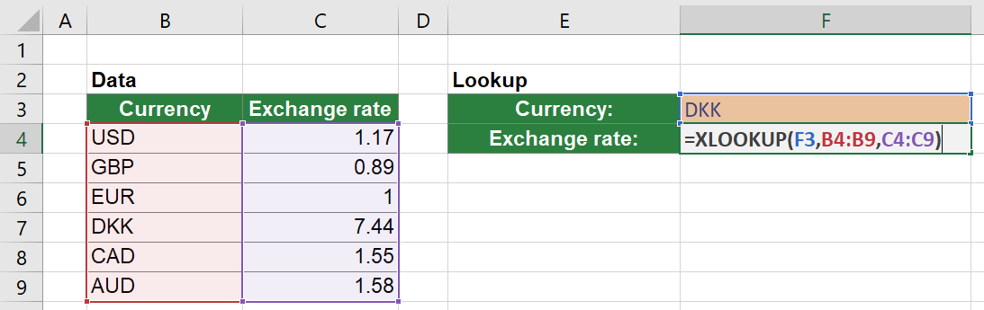
The first example is quite simple: You want to look up a currency exchange rate in a simple table as shown in the screenshot. In this example, you look for Danish Krones (DKK).
So, you look for DKK which is written in cell F3 within the cell range of B4 to B9. That means that these are your two first arguments already. Then, as the third argument, you just specify the return area – from which cell range do you want to get the return value? In this case, it’s in cell range C4 to C9. As a result, the function is “=XLOOKUP(F3,B4:B9,C4:C9)”.
It’s simple, isn’t it? Especially when comparing to VLOOKUP…
Example 2: Basic XLOOKUP for horizontal lookups
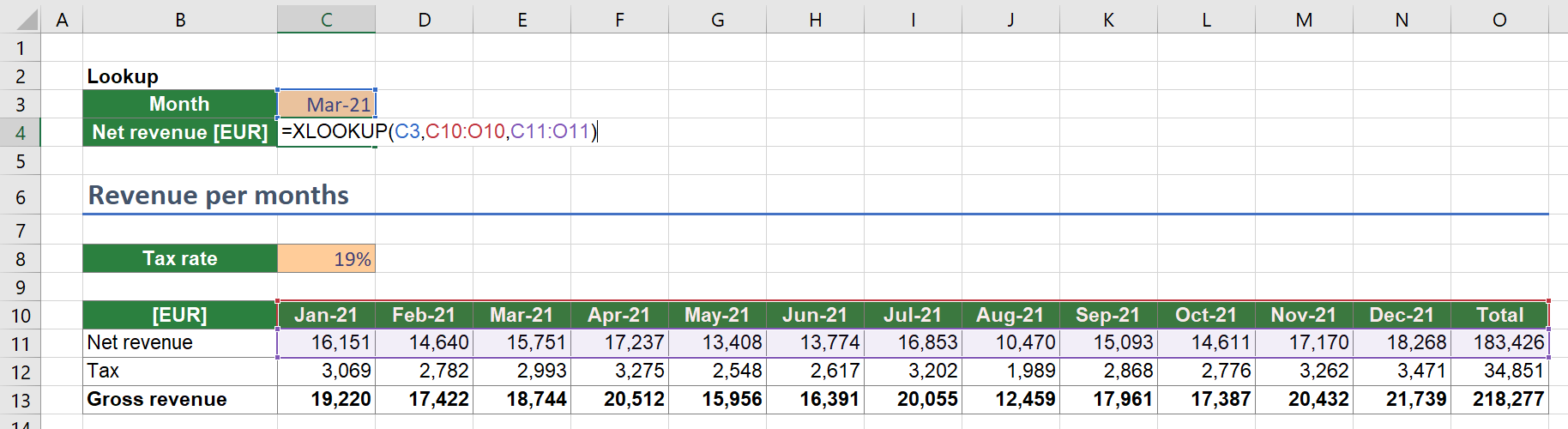
Our next example is also easy. The only difference is that it works horizontally. Assuming that you have monthly revenue values as shown in the screenshot below:

The arguments for the XLOOKUP function are as follows:
- The first argument is the search value. So, what do you search for? It’s the month, in this case provided in cell C3.
- Second argument is the search array. Where do you search in? It’s the month names in the headline of the date, cell range C10 to O10.
- And last: What value do you want to get returned? The revenue is in row 11. So the return range is C11 to O11.
Putting everything together leads to function =XLOOKUP(C3,C10:O10,C11:O11).
Example 3: XLOOKUP for multiple search criteria
If I might criticize the XLOOKUP function a little bit: That’s the only thing that isn’t really solved yet when it comes to the disadvantages of VLOOKUP and INDEX/MATCH. Searching for multiple criteria still works the same way as before: Concatenate the search criteria and insert a new search column (or row, depending on your lookup direction).
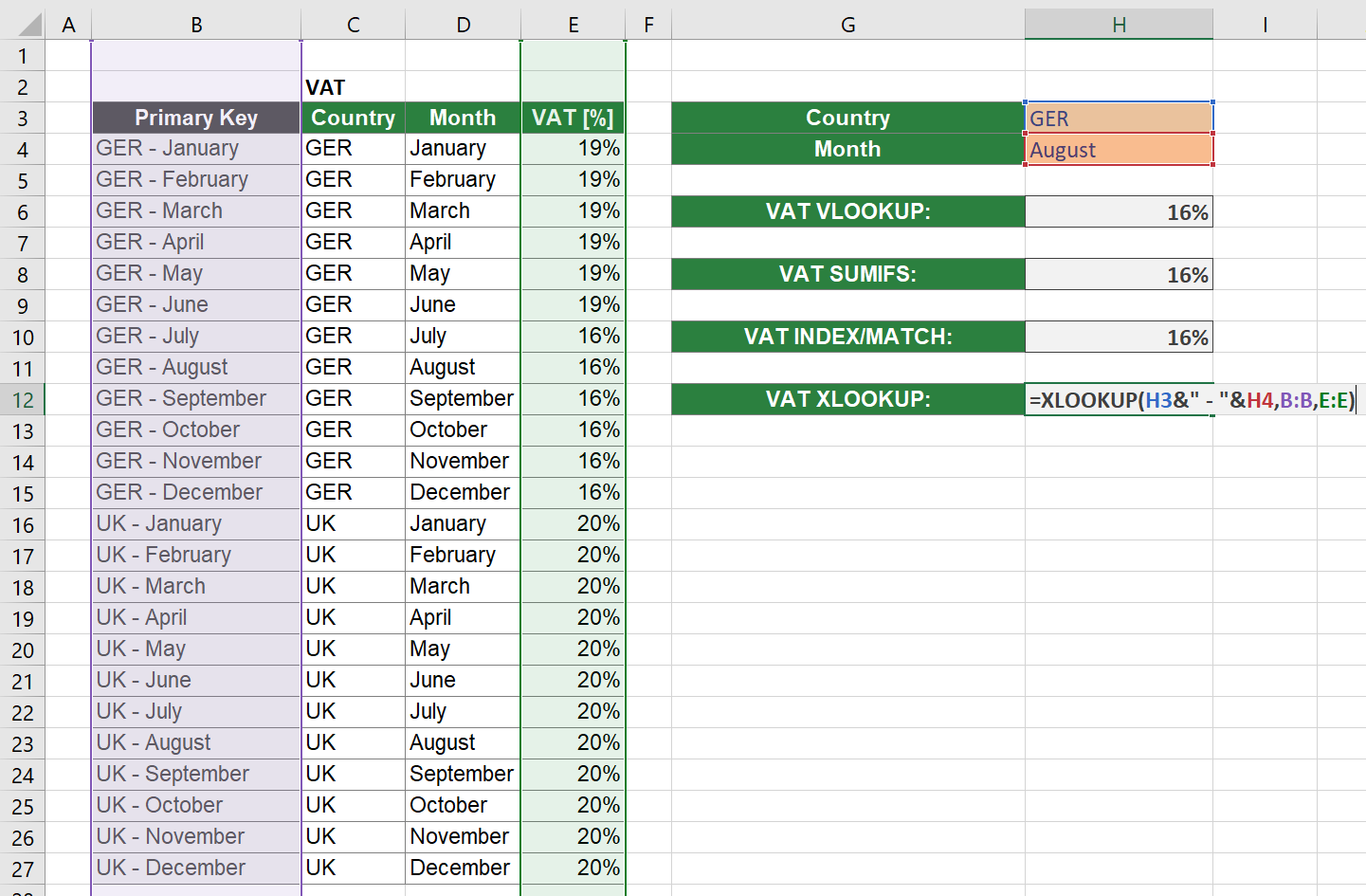
The example is as follows: You have a table of VAT rates per month and country. Depending on a selected month and country, you want to return the respective VAT rate.

Let’s explore it step-by-step:
- First you have to create a new column with the new “Primary Key”. This is a combination of Country and Month (concatenated by the & sign). So, the formula in cell B4 is “=C4&” – “&D4″. Please note: I’ve separated the two keys with ” – “. This way I always make sure that not by coincidence keys exist twice.
In worst case, the first part of the key could be “ab” and the second part “cd”. If I have another row with “a” and “bcd”, a simple concatenation would lead to “abcd” in both cases. That’s why I always put a separator in-between. - The XLOOKUP function works as always, with one difference: The search value must be the same concatenated value as in the primary key column.
When we put these things together, the XLOOKUP function is: “=XLOOKUP(H3&” – “&H4,B:B,E:E)”.
For comparison, I’ve also included solutions using VLOOKUP , SUMIFS and INDEX/MATCH.
Download
Please feel free to download all examples from above in this notebook. Follow this link and the download starts right away.
