Custom Number Formats in Excel: Everything You Need to Know!

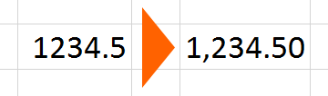
Excel provides many default number formats. But often, these formats are not enough. That’s were custom number formats come into play. Let’s take a look some examples:

• You want to display number in thousands or millions?
• Or have a thousands separator for percentage values?
• Or show a plus sign for positive values?

In such case, you need to create a custom number format. In this article, you learn everything you need to know. For making it easier for you, please feel free to download the example Excel file or the handy custom format card for printing it out.

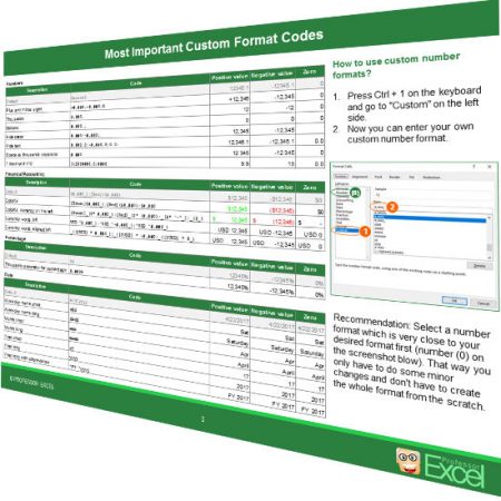
How to use custom number formats?

Inserting a custom number format in Excel is very easy:

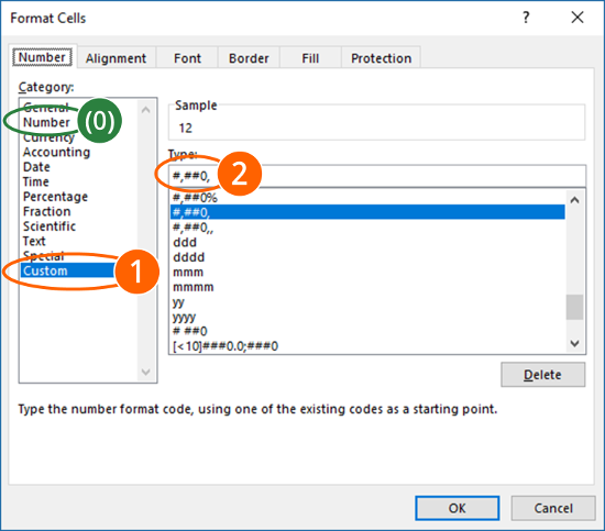
1. Press Ctrl + 1 on the keyboard and go to “Custom” on the left-hand side.
2. Now you can enter your own custom number format code.

Recommendation: Select a number format which is very close to your desired format first (number (0) on the screenshot). That way you only have to do some minor changes and don’t have to create the whole format from the scratch.

How do custom formats work?

Structure of custom number formats

If you create a custom number format, you have to regard some rules. A custom number format can be only a few characters or a long text string. They have at least one and at most four parts. Here are the four parts:

• Each part is divided by the ; (semicolon).
• A number format must at least have one part. All other parts can be omitted. If omitted, the first part counts for the later numbers. For example: You just define the positive number format. This formatting will be used for negative values, zeros and text (as far as possible).
• In practice, the fourth part is hardly used.

Let’s go through the 4 sections:

1. The first part is used for defining positive numbers. Also, if the following parts aren’t used, this format is used for negative number, zeros and text too.
2. Second part: If you want, you can define a different number format for negative number.
3. Do you want to have a special format for zeros? You can set it in the third section of the format code.
4. The fourth part is used for text. If there is no fourth part (and therefore no third semicolon) text will be shown normally. But if you use the fourth part, use the @ sign for showing it. If you don’t insert the add sign, text won’t be displayed.

Important basics for the shortcuts

Sign	Description	Code	Before	After
#	Add a # for a normal number. The digit won’t be displayed, if there is a preceding zero.	#,##0	123 1234 1234.5 0.123	123 1,234 1,235 0
0 (zero)	Add a 0 (zero) if there should for sure be a digit displayed, even if it’s a zero.	00000	123	00123
%	Add the percentage sign % if you want to display a number as percentage.	0%	0.8	80%
	Don’t use any sign if you want to hide number. Please note: You need at least one semicolon, otherwise Excel will interpret it as “General”	;	123
,	Insert a thousands separator. You can use this for showing numbers in thousands or millions as well (scroll down for more information).	#,##0	1234	1,234
.	Insert a decimal point in a number.	0.0	123	123.0
[Red]	Uses red color.   Please note: Conditional formatting rules offer much more color options.	[Red]	123	123
?	If you want to align the decimal points, use the question mark. Question marks can also be used for fractions.	???.??? 0 ???/???	12.345 1234.5 12.34	12.345 1234.5   12 17/50
“abc”	Within quotation marks, you can add any text.	“USD “0.0	123.45	USD 123.5
@	The @ sign is only used in the fourth section of the format code. Use it, if you want to display text in a cell. If you don’t use it (but still have 3 semicolons and therefore 4 sections), text will be hidden.	@”!”	Some text	Some text!

Steps for creating your own custom number format

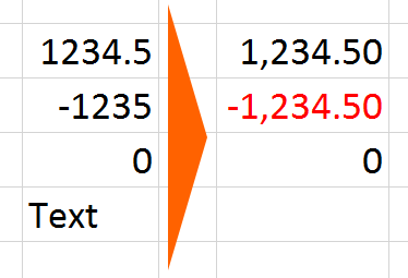
There are 3 steps for creating your own custom number format. The idea is to do it as simple as possible and therefore utilize built-in features. The 3 steps are shown with the example on the right-hand side. You want to create a custom number format, which

• uses thousands separators and 2 decimals,
• highlights negative number in red font color,
• displays 0 with no decimals and
• hides text.

Step 1: Choose a number format in the “Format Cells” window

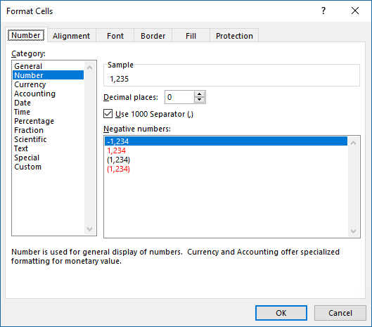
As the first step, choose a built-in number format which is very close to the one you eventually want to create.

1. Open the “Format Cells” window by pressing Ctrl + 1 on the keyboard.
2. Go to “Number“.
3. Check the tick of the thousands separator and change the decimal numbers to 2.
4. Click on “OK“.

If you open the “Format Cells” window again and click on “Custom” on the left-hand side, you’ll see the format code. In this example it should be #,##0.00 .

Step 2: Further modify the number format

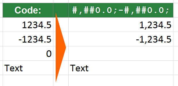
In this example, you want to further modify the number format for negative values, zeros and text. You continue with the code #,##0.00  created in step 1 above. If there is just one section, the format code is used for all kinds of values: For positive values, negative values, zeros and text because there is no particular definition for negative numbers, zeros and text.

• For negative values, you want to use the minus sign and use red color.
  • Copy the format code to create a second section. Now you got the format code #,##0.00;#,##0.00 .
  • Add the minus sign to the second part. #,##0.00;-#,##0.00 .
  • Add the code for red color for negative values: #,##0.00;[Red]-#,##0.00 .
• Zeros should just have one digit.
  • Add a third part to the code above by inserting a semi-colon at the end: #,##0.00;[Red]-#,##0.00;
  • As there should only be one digit, type “0”. #,##0.00;[Red]-#,##0.00;0
• For a text value, you want to show nothing.
  • Add a forth part to your code and leave it blank. That way, no value will be shown for text.
  • You custom format code now is #,##0.00;[Red]-#,##0.00;0; .

Step 3: Fine-tune the number of decimals

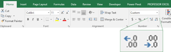
In the last step, you can further fine-tune the number of decimals. Therefore, use the buttons “Increase Decimal” or “Decrease Decimal” in the center of the “Home” ribbon.

Most popular codes

You don’t want to create your own code but just copy & paste one of the most popular custom number formats? Here are the most frequently asked codes.

Thousands + Millions

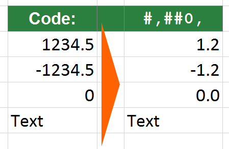
In many Excel tables, you can see divisions by 1000 or multiplications by 1000 in order to convert values to thousands or millions. An easier and more reliable way is to always use total values and just display them as thousands or millions.

The easiest way: Add a comma “.” to your code.

If you got this code #,##0  just add a comma “,” and you got #,##0, . That way, 2,345 becomes 2.

For more information about thousands and millions, please refer to this article.

Plus sign for positive values

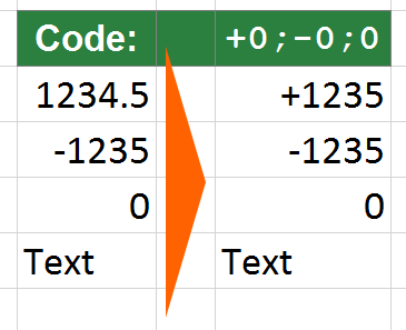
You want to show the plus sign for positive values? For example in charts? Use this code:

• +0;-0;0  for the following format: +1234 for positive values, -1234 for negative values and 0 for zeroes
• +#,##0;-#,##0;0  for the following format: +1,234 for positive values, -1,234 and 0 for zeroes.

Thousands separator for percentage

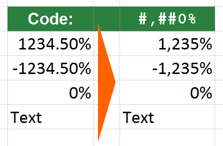
Sometimes, you got percentage values larger than 1000%. Excel doesn’t provide a thousands separator for such numbers. The following format adds the thousands separator:

#,##0%

Hide zeros

There are several ways to hide zeroes in Excel. Please refer to this article for more information about the other methods.

If you want to hide zeros with a custom number format, make sure to use a third part of the number format and leave it blank. Some examples:

• You got this code before: 0 . This is the default number format. In this case you have to add two parts (the second part handles negative values and the third part zeros): 0;-0;
• You got this code before: #,##0;-#,##0.  Use a third part by just adding a semicolon. #,##0;-#,##0;
• For percentage numbers: 0%;-0%;

Weekday name, name of the month, number of the year

Do you want to show a weekday name of a given date? You could either do this with formulas or just display the weekday name of a date cell. Use the following codes:

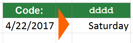
• Weekday
  • ddd  for the abbreviation: the date 04/21/17 will be shown as “Fri”
  • dddd  for the full name: the date 04/21/17 will be shown as “Friday”
• Month
  • mmm  for the abbreviation: the date 04/21/17 will be shown as “Apr”
  • mmmm  for the full name: the date 04/21/17 will be shown as “April”
• Year
  • yy  for just the last two digits: the date 04/21/17 will be shown as “17”
  • yyyy  for the full year number: the date 04/21/17 will be shown as “2017”

Tips and tricks

• Some formatting can also be done by conditional formatting rules. If your custom number format becomes too complex, please switch to conditional formatting rules. They are usually easier to use and provide more options.
• Use copy and paste as often as possible. Either for the formatting itself, or for the custom number code. That way, you can save a lot of time.
• Do you want to change the thousand separator, for example use a full stop instead of a comma? You could achieve this either in the “Region” settings of Windows or override the thousands and decimal separator in Excel. Please refer to this article for more information.

Free Download

As a gift for you, please feel free to download these files:

• A handy printout with the most common custom format codes. It’s a one-page PDF file. Download it here.
• The same codes as an Excel table. Maybe it’s easier for you to copy & paste the formats. Download it here.

Was the information in this article helpful? Why don’t you sign up for our free, monthly Excel newsletter?

One more recommendation for custom number formats

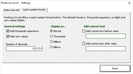
With our Excel add-in “Professor Excel Tools”, you can create your favorite number format. Even better, you can apply it with just one click. Why don’t you give it a try?

Image by Pexels from Pixabay