


Until Excel 2016, there is no built-in MINIF-Formula in Excel. There are COUNTIF, SUMIF, AVERAGEIF but no MINIF nor MAXIF before the latest version. However, there are situations in which you need to get the minimum under a condition. In the following post, we are going to illustrate how to returnthe minimum using a simple example. We got an Excel table with two columns “Car type” and “Price”. We want to know the minimum price for each car type. Sounds easy? Unfortunately, Excel makes it unnecessarily difficult to calculate.
Some introductory words…

There are many different ways of getting the minimum value under a condition. For example, sorting the whole table and using a “VLOOKUP”, which will return the first value. But as this method is quite unstable, we are going to look at 5 more stable alternatives.
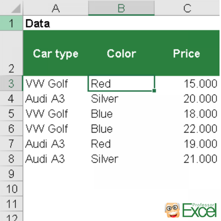
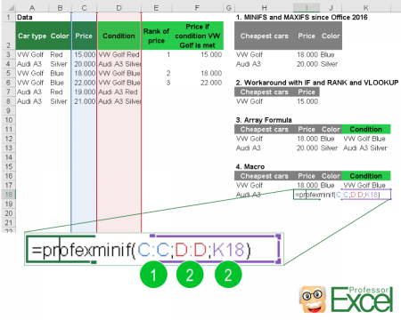
All the methods will be demonstrated with a simple example: We got three columns: The car type in column A, the color and the price (as shown on the picture on the right hand side).
Method 1: The easy way – MINIFS and MAXIFS formulas

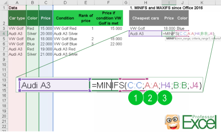
Since Office 2016, Microsoft finally introduced built-in MINIFS and MAXIFS formulas. So the bad news is: If you don’t have the latest version of Excel, you can’t use these formulas. Furthermore, you have to make sure that everybody who works on your file should have Office 2016 as they otherwise will get #NAME? errors.
MINIFS and MAXIFS work pretty much the same way as SUMIFS. The formula has at least three parts:
- The minimum (or maximum) range: In this range, Excel will search for the minimum or maximum value and return it.
- The first criteria range: The range of cells which contain the first criteria.
- The first criteria: This is the value, which Excel searches for in the first criteria range.
If you got more criteria, you can just extend the formula and repeat number 2 and 3 from above. Let’s take a look at an easy example: We got car names in column A, their colors in column B and their prices in column B. We want to know the lowest price of a blue VW Golf:
=MINIFS(C:C,A:A,"VW Golf",B:B,"Blue")For more information on the MINIFS formula, please refer to this article provided by Microsoft.
Method 2: The workaround – inserting support columns and use the rank formula

If you don’t want to go with VBA or array formulas, there are workarounds for getting the minimum or maximum value under one or more conditions. Let’s take a look at one of them.
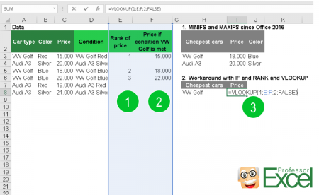
The basic idea is to only show the values which the conditions apply for. Then we use the rank formula for identifying the smallest (or largest in case) and return the corresponding value with a simple VLOOKUP.
We start by adding two columns:
- Column E contains the rank of the values in column F. We put this in column E in order to use a simple VLOOKUP later on. If you are willing to use the INDEX/MATCH combination, you are free to choose their sequence. The formula in our case looks something like this:
=IFERROR(RANK(F3,F:F,1),"")
The RANK formula returns the rank of value F3 among all values in column F. The number one determines, that the smallest value gets the number 1. In case of a blank cell, we avoid an error message by wrapping the IFERROR formula around our RANK formula.
- The column F contains an IF formula. If our conditions are met, the price will be shown. So formula looks like this:
=IF(A3="VW Golf",C3,"")
- The VLOOKUP just looks for the number 1 in column E, as this indicates that there is the smallest value. It’ll return the corresponding price from column F.
Do you want to boost your productivity in Excel?
Get the Professor Excel ribbon!


Add more than 120 great features to Excel!
Method 3: The complicated way – get MINIF and MAXIF with an array formula

First: What is an array-formula? Well, Microsoft provides this answer:
An array formula is a formula that can perform multiple calculations on one or more of the items in an array.
Array formulas are being used like normal formulas: You type the formula as usual. But instead of pressing enter, you press Ctrl + Shift + Enter. That’s why they are sometimes referred to as “CSE” formula. Along with the advantage of being able to perform more powerful calculations, one disadvantage is, that you can hardly change the size of the ranges once the formula is created. Inserting or deleting a row or column later on is not possible. Array formulas can be recocnized by the “{” and “}” embracing the actual formula.
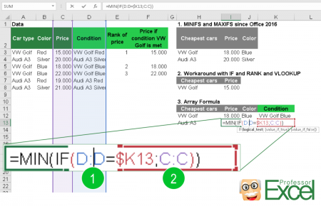
The formula for the MINIF is quite short:
=MIN(IF(D:D=K13,C:C))
After typing this formula, press Ctrl + Shift + Enter and the { and } are added automatically. In this example, you should see the result as shown in the picture on the right hand side. Getting the maximum value under a condition works the same way, except that you have to replace MIN with MAX.
Method 4: Programming: Get the minimum value under a condition with a VBA macro
As usual, you can also solve this problem with a VBA macro. Therefore, go to Developer. Click on Editor, right click on Microsoft Excel Objects and insert a new module. Paste the following code into the new module:
Function PROFEXMinIfExample(MinRange As Range, ConditionRange As Range, ConditionCell As Range)
    'This function returns the minimum of a range of cells meeting one condition
    'The order of arguments:
    'PROFEXMinIf(the range with the value to be returned, the range for comparing a condition, the condition as one cell)

    Application.Volatile
    'Refresh formula with every time calculating

    Dim minimumValue As Double
    'The minimum value will be saved here. In the loop later, it will always be overwritten, when a smaller value is found

    Dim i As Integer
    i = 0
    'A variable for counting, set to 0

    Dim cell As Range
    'Use the variable "Cell" later on for going through ranges of cells

    Dim firstValue As Boolean
    firstValue = True

    For Each cell In ConditionRange
    'Go through all cells in the condition range

        If ConditionCell = cell Then
        'Checking for the condition. If the condition is met, continue

            If firstValue = True Or MinRange(i + 1, 1) < minimumValue Then
            'Check next, if either it is the first value under the given condition or if the current value is smaller than
            'the value saved to minimumValue
            'i+1 because we are starting with "0" for i

                If MinRange(i + 1, 1) <> "" Then
                    'If the current cell is not blank

                    minimumValue = MinRange(i + 1, 1)
                    'Save the current value to minimumValue

                    firstValue = False
                    'Because next time in the loop, it's not the first value any more, we have to set
                    'first value to false
                End If
            End If
        End If
        i = i + 1
        'Increase i by 1 so that with next loop we are looking at the next cell
    Next

    PROFEXMinIfExample = minimumValue
    'Returns the minimum value

End Function
For displaying the minimum value under a condition, you just have to type the following formula
=PROFEXMinIfExample(C:C,D:D,K17)
This formula can be divided into three parts:
- The range containing the value, you want to get returned. In our case, it’s the price of a VW Golf.
- The range which has to meet the condition. For us, that means all cells with “VW Golf” in it.
- The condition: Either a cell reference, for example D8 which contains the name “VW Golf” or the condition itself.
In our example, the lowest price for a Golf is 15,000 and 19,000 for a Audi A3.
How to deal with several conditions? The easiest way is to combine them into one cell. For instance, we got one more column with the color of the cars. We can combine the type and the color into another new column. Just type =A3&A4 into cell D3 and use this as the new condition.
By the way: MAXIF works the same way, just modify it within the code (replace ‘<‘ by ‘>’).
Method 5: The expert way – use the Excel add-in ‘Professor Excel Tools’
As getting the MINIF or MAXIF to work is quite difficult we thought of an easier way to use it: We integrated the MINIF- and MAXIF formulas into our Excel add-in ‘Professor Excel Tools’.
- Go to the ‘Professor Excel’ ribbon.
- Click on Formula within the ‘Quick Cell Functions’ group.
- Select PROFEXMinIf or PROFEXMaxIf and follow the instructions.
Please try ‘Professor Excel Tools’ for free: Just click the download button below and activate it within Excel.


This function is included in our Excel Add-In ‘Professor Excel Tools’
(No sign-up, download starts directly)
More than 35,000 users can’t be wrong.
Download
Please feel free to download all the examples from above within one comprehensive Excel sheet. As there is also the 4th example included, it has to be a .xlsm file. Don’t worry – in case Excel asks you – there is no virus but just the code from above.
Please click here for downloading the example.