LOOKUP Function in Excel: How to use & why to avoid it!

Besides the well-known VLOOKUP function, there is a similar function in Excel: LOOKUP. The function is very unknown and hardly used. But there are good reasons why you should not use the function. Let’s start with the basics about the function and then talk about why you should avoid it.

Before we start with the LOOKUP: If you consider using it in Excel – don’t! Rather take a look at the new XLOOKUP function. Or INDEX/MATCH. They usually work much better. That said: Let’s get started!

Vector form of the LOOKUP function

Structure of the function in the vector form

The LOOKUP function is available in two forms, a vector form and an array form. Whether you use the vector or array form of the function is determined by the size of array and the number of arguments.

The LOOKUP function in the vector form has two arguments and one optional third argument. The structure of the function looks like this:

1. The lookup value is the value you search for. As usual, it can be a number, text, logical value, name or cell reference.
2. The lookup vector defines the cell range you search the lookup value (1) in. In the vector form it can only be a one-dimensional cell range. That means either a cell range within one row or within one column.
3. The result vector is optional. If you want to return a value from another column or row than the lookup vector, you can define it here.

Curiosities about the function

There are some curiosities about the this formula:

• If your search value can be found several times in the lookup vector, it returns the last instance.
• In case the result vector doesn’t have the same size like the lookup vector, there are two possibilities:
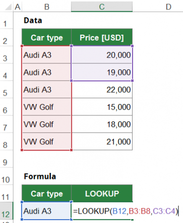
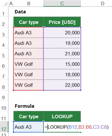
  • If the result vector still indicates its shape (e.g. horizontal, vertical), Excel will still try to get the correct result although it’s outside of the result vector. The image on the right-hand side shows such example: Excel wants to return the third value (the last time Audi A3 is listed in the cell range B3:B8). It won’t regard the exact size of the result array – just the starting cell (C3) and its direction (vertical). This function still returns 22,000.
    Furthermore, you can move the result vector, for example to C2:C3. That way, the LOOKUP function returns the third value starting from C2 – which is 19,000.
  • If the third argument – the result vector – doesn’t show the direction (because it’s just one cell) or has a different direction than the LOOKUP vector (e.g. horizontal whereas the LOOKUP vector has a vertical shape) it will assume the array form of the LOOKUP vector and return the lookup value.
• You must sort your lookup vector in ascending order. Otherwise you receive an #N/A error message. It’s the same error message if your search value can’t be found.

Example for the LOOKUP function in the vector form

The picture on the right-hand side shows an example for the vector form of the LOOKUP formula.

1. The first argument is the lookup value and in the example, it refers to cell B12. Cell B12 has the car type “Audi A3”.
2. The second part of the LOOKUP formula defines the lookup vector. In this case, it’s the cell range B3 to B8.
3. The third and last argument of the vector form of LOOKUP is the result vector. In this example, it’s the cell range C3 to C8.

In summary, you search for “Audi A3” in the cell range B3 to B8. If found, the corresponding value from the cell range C3 to C8 will be returned.

Which value will be returned in this case? The result is 21,000. Why not 20,000 as it’s the return value to the first instance of “Audi A3”? Because of the curiosity of the LOOKUP formula that it returns the from the last instance the search value is found. And that’s the case in cell B5. But careful: If cell B8 also contains “Audi A3”, still 21,000 will be returned. That’s due to the last curiosity, that the lookup vector must be sorted in ascending order.

Array form of the LOOKUP function

Structure of the function in the array form

The array form of the formula only has two arguments unlike the vector form, which has an additional, optional third argument.

The structure of the function in the array form:

1. The lookup value is, like in the vector form, the value (number, text, etc.) you search for.
2. The array encloses both: The search row or column and the return row or column. Why row or column? Because the shape of the array defines if the LOOKUP formula searches vertically or horizontally. If the array has more rows than columns, it searches vertically. If the array has more columns than rows the other way: it searches horizontally.

How does Excel know, which column (or row) to return as there are only two arguments? It’s quite straight forward: If your LOOKUP function works vertically (that means your array has more rows than columns) it searches the lookup value in the leftmost column. It returns the value from the rightmost column in your array.

Example for the LOOKUP formula in the array form

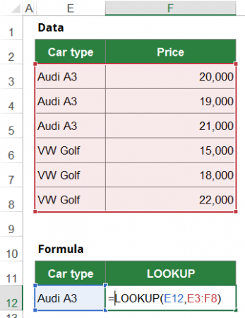
The image on the right-hand side shows an example for the array form of the LOOKUP formula. The formula in cell F12 has two arguments:

1. The search value is provided in cell E12. In this case, you search for “Audi A3”.
2. The array is the cell range E3 to F8. That is the highlighted range of cells above. Because this range has more rows than columns, the LOOKUP formula works vertically. It searches in the leftmost column of this range, which is the column E. It returns the value from the rightmost column in this cell range which is column F.

What is the result of the formula? Like in the example of the vector form of the formula it’s 21,000. That is the corresponding value of the last time Excel finds “Audi A3” in the cell range E3 to E8.

Please note: If your array is square (that means it has the same number of rows and columns), it works vertically.

Determine the form of the function

• The formula has three arguments: Vector form of the formula
• The formula has two arguments.
  • The second argument is a one-dimensional cell range (for example just covering cells within one row or column): Vector form of the formula.
  • The second argument is a two-dimensional cell range: Array form of the formula.

Troubleshooting: Typical errors

If your LOOKUP formula doesn’t return the expected result, please check one of the following typical errors.

• You receive an #N/A error message? Either your search value really can’t be found or you haven’t sorted the lookup array in ascending order.
• Wrong result
  • In the array form of the LOOKUP formula, the shape of the search array determines the search direction.
  • In the vector form, the last occurrence will be returned.

Recommendation: Use INDEX/MATCH or VLOOKUP/HLOOKUP instead.

Why you should avoid the LOOKUP formula

• Microsoft strongly recommends in the help section of the function to use VLOOKUP (or HLOOKUP) instead of LOOKUP. Especially the array form of the formula is only provided for compatibility reasons with other spreadsheet programs.
• The function is very unstable. So just adding a row or column can completely change the why it works (vertically, horizontally, array or vector form).
• Despite its few arguments, LOOKUP is (for most Excel users) much more complicated than VLOOKUP, HLOOKUP or INDEX/MATCH.

Image by ThePixelman from Pixabay