One of the basic applications in Excel is summing up values. The most popular ways of adding up numbers are just using the ‘+’ sign or the formula SUM. But there are many other methods. Do you know about these 6 other ways to sum up values in Excel? In this article we’ll take a look at 8 methods for summing up values in Excel and compare them.
8 methods in detail
Let’s start by taking a look at each method to create sums in Excel separately. After that we will compare them by their most important characteristics.
01. The most popular way: SUM()
The SUM() formula is extremely easy to use: Just type =SUM() into an empty cell or press the sum button on the right hand side of the Home ribbon. Within the brackets you’ve got several options:
- Write the “hard coded” values (although not recommended), e.g. =SUM(3,5). The return value will be 8.
- Instead of hard coded values you can also refer to other cells, e.g. =SUM(A1,A2). The sum of the values in these two cells will be returned. Also getting sums of larger cell ranges is possible: =SUM(A1:A5) will return of all cells A1, A2, A3, A4 and A5.
Please note that the sum of all cells within the given cell range will be added. If you hide cells in between or cells are invisible because you’ve set a filter, they are still regarded.
02. The easiest way: ‘+’ sign
Very intuitive: Using the ‘+’ sign. Like the SUM() formula, you got the two options of combining two values with the ‘+’ sign (e.g. =3+5) or cell references (e.g. =A1+A2).
Please note that the ‘+’ sign can’t regard cell ranges but only single cells or values. That fact makes this method more troublesome but also more stable at the same time: As you have to select any input cell separately, you won’t have the problem that you accidentally regard unwanted values when inserting rows or columns in between.
03. The fastest way: Checking the status bar

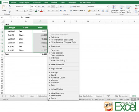
If you select data in Excel, usually a summary of the selected data is already shown in the status bar. It’s located on the bottom of the window on the right hand side.
If there is no sum shown, check these two options:
- Is your data really numeric values? Or is it formatted as text? This article has more information on forcing text cells to a number format.
- Have you defined that you want to see the sum in the status bar? Right click on it and check if ‘Sum’ is ticked. If not, click on it for setting the tick.
04. The old way: SUMIF or SUM(IF())

Before there was the SUMIFS formula, Excel provided a similar way for adding values under a condition: SUMIF (without ‘s’ in the end). SUMIF works more a less the same way as SUMIFS but can only regard one condition at a time.
If you are familiar with SUMIFS, we recommend only using SUMIFS from now on. If you are not familiar with SUMIFS continue with the next method – and forget about SUMIF…
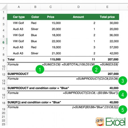
Some more words about =SUM(IF()). With such array formula you can also sum up values under a condition. Let’s say, we want to know the sum of the prices of all blue cars in the picture on the right hand side. The formula would look like this:
{=SUM(IF(B3:B8="Blue",C3:C8,0))}Type the formula without the curly brackets. Instead of just pressing enter press Ctrl + Shift + Enter. That way, you can also combine conditions by adding another IF formula within the first IF formula.
05. The new and better way: SUMIFS
SUMIFS is only available since Excel 2007 – but nowadays most people use Excel 2007 or above. SUMIFS sums up all values under one or more conditions. It can be used for getting a sum of values but also for just looking up values – as long as those values have a numeric format. Please refer to this article for more information on how to use the SUMIFS formula.
06. The complicated way: SUMPRODUCT
SUMPRODUCT can sum up values as well. But it can do much more than just returning sums:
- SUMPRODUCT can multiply two columns (or rows) with each other and return the sum (number 3 in above picture).
- Furthermore SUMPRODUCT can regard criteria. It’s a little bit more complicated than just with SUMIFS. Number 4 in above picture has an example for adding a condition to the SUMPRODUCT formula: In this case the sum of all blue car prices will be returned.
As the usage of SUMPRODUCT is comparatively difficult, it’s recommended to use other ways:
- For simple sums, go with the SUM formula.
- A sum of the product of two columns can easily be done with a third column, which contains the product of the two original columns.
- For getting a sum under conditions please take a look at the SUMIFS formula (method 5 above).
07. The ‘only visible’ way: SUBTOTAL
SUBTOTAL has two options: Regarding all cells or only visible cells. Now we concentrate on the only visible cells as it is the major difference to the other methods. Hidden cells – for example because they’ve been filtered – won’t be regarded. There are a number of possible calculation methods and one of them is summing up the values.
The SUBTOTAL formula has two parts (please compare to number 2 in the image above):
- The type of calculation. For summing up values just type 9 (if you want to regard all cells) or 109 for the only visible cells.
- The cell references containing the values to be added. There can be hidden cells, rows or column within this range – they won’t be regarded in the result.
Do you want to boost your productivity in Excel?
Get the Professor Excel ribbon!


Add more than 120 great features to Excel!
08. The Pivot Table
If you just want to get a simple sum, a Pivot Table might be a little bit over the top. But anyway, a Pivot Table can add up values. Actually, with a Pivot Table you can do many more things:
- You can summarize data by any of the fields in your table.
- Also, you can conduct calculations.
- You can count, sum up, create averages and much more.
We’ve already published various articles about Pivot Table:
- Have a look at this article if you want to know how to set up Pivot Tables.
- Refer to this article if you want to know how to change the data source of a Pivot Table.
- This article show you how to work with large data and PowerPivot.
- You are annoyed by the always changing column widths after each update of y0ur Pivot Table? Take a look at this article.
Comparison
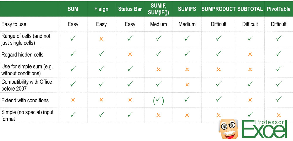
After getting to know each method in detail, we can compare them. The criteria are:
- Easy to use: Is the application easy or rather difficult?
- Range of cells (and not just single cells): Does this formula or function regard a range of cells or do you have to type each cell reference individually?
- Regard hidden cells: Are hidden cells being regarded?
- Use for simple sum (e.g. without conditions): Is it possible to create a simple sum – and not only sophisticated calculations with conditions and so on?
- Compatibility with Office before 2007: There were new formulas and functions introduced with Excel 2007. The default file format changed from .xls to .xlsx. Are these methods compatible with the old versions of Excel?
- Extend with conditions: Can you use conditions for creating the sums?
- Simple (no special) input format: Is a special input format required, e.g. conditions in one column or proper headings in case of a Pivot Table?