Today, we got a quick tip for you: Sort data left to right. Most Excel users don’t know that it is possible to sort horizontally. Admittedly, the option is a little bit hidden in Excel. But once you know it, it’s not a big deal.
As the option for sorting data left to right is a little bit hidden in Excel, most users either drag and drop rows manually or transpose them first. But that’s not necessary! There is an easy method letting Excel sort your data horizontally for you.
Do these steps to sort horizontally
Actually sorting data left to right in Excel is quite simple. You just have to change the Sort Options from “Sort top to bottom” to “Sort left to right”.

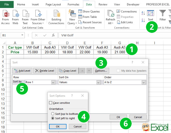
The example: You got the simple table as shown in the image on the right hand side. Row 1 contains cars (here just shown by their type) and row 2 has the corresponding price. You want to sort the table by the car type.

Follow these steps:
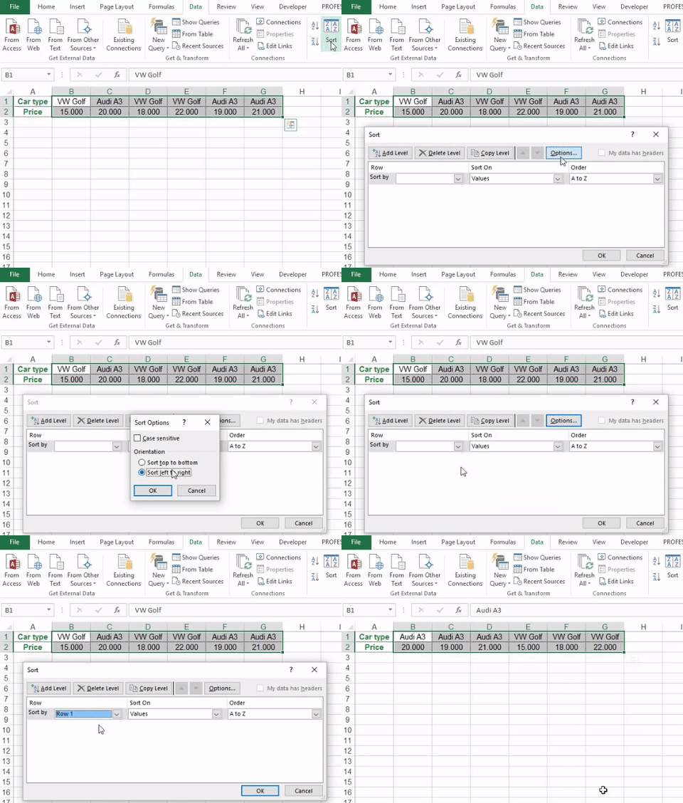
- Select the data you want to sort. Important: Don’t include the title column (here: column A) in your selection. When you sort horizontally, the option “My data has headers” is greyed out.
- Click on Sort within the Data ribbon.
- Click on Options in the Sort window.
- Select “Sort left to right” instead of “Sort top to bottom”.
- Select your search row. In our example we sort by the car type in row 1.
- Confirm with OK.
Please note: Excel saves your last selection. Next time you want to sort a table top to bottom you have to switch the sort direction back to “Sort top to bottom”.
Animation
The complete process one more time as an animation. Keep in mind, that you should not include the title column (column A) in your selection.

Do you want to know more about sorting options in Excel? We’ve already published articles for basic sorting knowledge and how to use filters or advanced filters. Also Pivot Tables offer a lot of sorting options.

