Check if Excel Cells Have the Same Value: 5 Easy Methods

Excel is like that versatile Swiss Army knife you didn’t know you needed—whether you’re balancing budgets, tracking your fitness progress, or planning your next vacation, it’s got your back. One common task you might encounter is verifying whether multiple cells contain the same value. Whether you’re double-checking data entries or ensuring consistency across your spreadsheets, knowing how to perform these checks efficiently can save you time and headaches. Let’s dive into five methods (and a bonus sixth!) to help you master this Excel trick with ease and maybe even a chuckle or two.

Method 1: Simple Comparison for Two Cells with =A1=B1

Description

When to Use

You have just two cells to compare and want a quick, straightforward answer.

How it Works

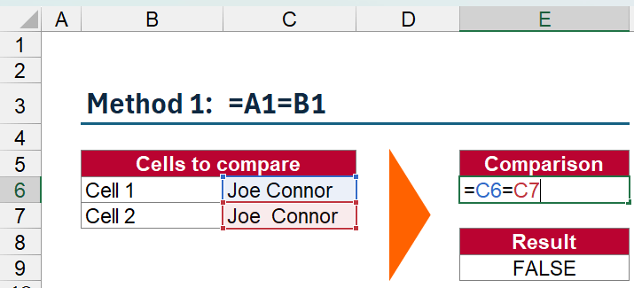
The simplest way to check if two cells are identical is by using the equality operator (=). For example, to compare cells C6 and C7 like in the screenshot on the right-hand side.

Pros and Cons

Pros	Cons
Simplicity: Easy to understand and implement.	Limited Scope: Only works for comparing two cells at a time.
Quick Feedback: Instantly shows whether the cells match.	Binary Output: Doesn’t provide details beyond TRUE or FALSE.

You want to return 0 and 1 instead of FALSE and TRUE? Just multiply by 1. So the formula in the example above would be:

=(C6=C7)*1

Method 2: Comparison for Multiple Cells with =AND(A1=B1, B1=C1, ...)

Description

When to Use

You need to compare more than two cells and ensure all match.

How it Works

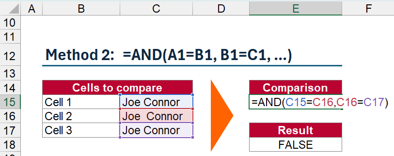
By nesting multiple AND functions, you can check if all specified cells are equal. For instance, to compare A1, B1, and C1:

Pros and Cons

Pros	Cons
Flexibility: Can handle any number of comparisons by extending the AND function.	Cumbersome for Many Cells: Manually adding each comparison can be tedious.
Logical Clarity: Clearly shows all comparison points.	Prone to Errors: Easy to miss a comparison when dealing with many cells.

Pro Tip: For larger ranges, consider using other methods to keep your formulas neat and efficient!

Method 3: Numeric Same Values Comparison with =AVERAGE(A1:C1)=MAX(A1:C1)

Description

When to Use

You’re dealing with numeric data and want a creative way to verify uniformity.

How it Works

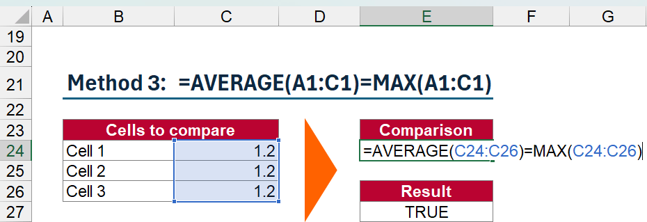
If all numeric values in a range are the same, the average will equal the maximum (and the minimum). Here’s how to implement it for cells A1 to C1:

Pros and Cons

Pros	Cons
Smart Use of Functions: Leverages Excel’s built-in functions creatively.	Numeric Only: Doesn’t work with text or mixed data types.
Minimalist Formula: Requires fewer comparisons than the AND method.	Indirect Comparison: Relies on statistical properties, which might be less intuitive.

Quick Insight: It’s like using the average score in a game to check if all players scored the same—if the average equals the highest score, everyone’s in sync!

Method 4: Utilizing the COUNTIFS Function

Description

When to Use

You need to verify if all cells in a range have the same value, especially in larger datasets, without manually specifying each comparison.

How it Works

The COUNTIFS function counts the number of times specific criteria are met across multiple ranges. To check if all cells in a range match the first cell, you can use COUNTIFS with each cell compared to the reference cell. Here’s how to implement it for cells A1 to C1:

• range: The group of cells you want to compare, in this case the blue range C33:C35.
• A1: The reference cell to match against – one of the values within the range to compare (here: C33)

Pros and Cons

Pros	Cons
Scalable: Easily handles large ranges without extensive formulas.	Reference Dependency: Relies on one cell as the reference, which might not be ideal in all scenarios.
Flexible: Can be adapted for various conditions and criteria.	Potential for Errors: If the reference cell is blank or contains unexpected data, results may be misleading.

Advanced Tip: Combine COUNTIFS with other functions like IF to create more dynamic and informative outputs. For example:

=IF(COUNTIFS(A1:C1, A1) = COUNTA(A1:C1), "All Match", "Mismatch Found")

This formula will return “All Match” if all cells in the range have the same value, and “Mismatch Found” otherwise.

Method 5: Using Excel Add-In Professor Excel Tools

Description

When to Use

You prefer a specialized tool for more advanced or streamlined comparisons.

How it Works

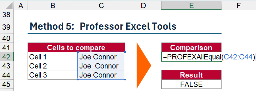
Professor Excel Tools is an add-in that simplifies various tasks, including cell comparisons. The key function for checking if multiple cells have the same value has three arguments:

1. Cell Range: The group of cells you want to compare.
2. Skip Blanks (optional): If set to TRUE, blank cells are ignored; otherwise, they’re treated as equal.
3. Case Sensitive (optional): If set to TRUE, the comparison distinguishes between uppercase and lowercase letters.

Formula Structure:

=PROFEX_EQ(range, [skip_blanks], [case_sensitive])

Examples

Range	Formula	Result
“Excel”, “excel”, “EXCEL”	=PROFEXAllEqual(A1:C1, TRUE, TRUE)	FALSE
“Data”, “Data”, “Data”	=PROFEXAllEqual(A1:C1)	TRUE

Pros and Cons

Pros	Cons
User-Friendly: Simplifies complex comparisons into a single function.	Requires Add-In: You need to install Professor Excel Tools, which might not be feasible for everyone. But: the formula functions in Professor Excel Tools are free to use – no subscription needed. Just download and install Professor Excel Tools.
Customizable: Offers options to skip blanks and enforce case sensitivity.
Efficiency: Handles large ranges effortlessly.

Expert Tip: If you frequently perform complex comparisons, investing in a robust add-in like Professor Excel Tools can save you countless hours in the long run!

Bonus Method: Utilizing Conditional Formatting to Highlight Cells with the Same Value

Description

When to Use

You want a visual representation of matching cells without using formulas.

How it Works

Conditional Formatting allows you to highlight cells that match a specific condition. To check if multiple cells have the same value:

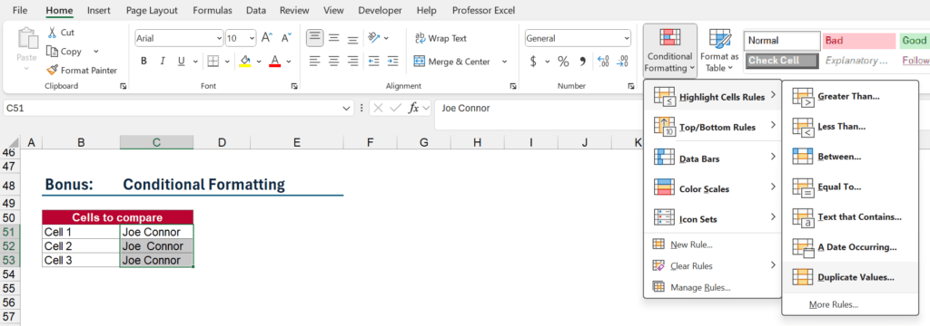
1. Select the range you want to compare (e.g., A1:C1).
2. Go to Home > Conditional Formatting > Highlight Cells Rules.
3. Choose “Duplicate Values…”.
4. Set your desired formatting (e.g., fill color).
5. Click OK.

Pros and Cons

Pros	Cons
Visual Aid: Instantly see which cells match through color coding.	Less Precise: Doesn’t provide a TRUE/FALSE output for further calculations.
No Additional Columns Needed: Keeps your worksheet tidy.	Complex for Large Ranges: Setting up rules for extensive data can be tricky.
Dynamic: Automatically updates as data changes.	Depending on your requirements, this approach might not be the perfect solution because it highlights all values that are duplicates.

Visual Hack: Think of Conditional Formatting as Excel’s way of giving your data a stylish makeover—highlighting what’s important without the need for extra formulas!

Conclusion for Checking, if Excel Cells Have Same Value

Checking whether multiple cells in Excel share the same value doesn’t have to be a daunting task. Whether you prefer straightforward formulas, clever function combinations, specialized add-ins, or visual highlights, Excel offers a variety of methods to suit your needs.

• Method 1 and Method 2 are perfect for quick, simple checks.
• Method 3 adds a numeric twist for those who love leveraging Excel’s mathematical prowess.
• Method 4 using COUNTIFS provides scalability and flexibility for larger datasets.
• Method 5 with Professor Excel Tools is ideal for power users seeking efficiency and customization.
• And let’s not forget our bonus method—Conditional Formatting—for those who like their data to look as good as it functions.

Whichever method you choose, mastering these techniques will enhance your data management skills and make your Excel experience even more powerful. So go ahead, give them a try, and watch as your spreadsheets become more consistent and reliable. Happy Excel-ing!

Download: Don’t forget to download the examples from above. Click here to start the download.