There are several ways for sorting data in Excel: Using filters, Pivot Tables or the built in function for sorting data. The sort function has the advantage that it’s easy to use and can be modified in detail. In this article we learn, how to apply the sort function in Excel.
How to sort data in Excel

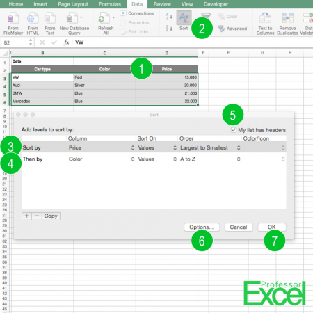
Sorting data in Excel is quite easy. The following numbered steps are corresponding to the picture above).
- Select the data that you wish to sort.
- Click on “Sort” in the middle of the Data ribbon.
- Select the first column that you want to get sorted. In this case, it is the price. You can define the order (e.g. Largest to Smallest) or what criteria you want get your values to sorted by (e.g. value, cell color, font color).
- If there are two items with the same value, you can define a second sort criteria.
- Did you select the header row in step 1? If yes, then make sure the corresponding checkmark is ticked.
- Under “Options” you can further define the sorting direction (vertical or horizontal).
- Confirm with “OK”.
Please note: Be careful that cell references to other rows within your data are not changed.
