The OFFSET formula is a very powerful formula, but unfortunately not easy to understand. It basically refers to another cell or cell range. You specify a starting point (“Reference”) from which you count rows and columns. If the starting point is cell A1 and you tell Excel to count 2 cells to the right and 3 down, it’ll return the reference to cell.
How to use the OFFSET formula
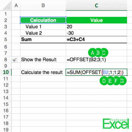
The OFFSET formula has five parts, of which the first 3 parts are required and the 2 last parts are optional (the letters are corresponding with the picture above):
- The reference: The initial cell or cells which we will start counting from (letters A and D in above example).
- The number of rows counting from the reference (letters B and E in above example).
- The number of columns counting from the reference (letters C and F in above example).
- Height: If you want to get a cell range and not just a single cell, you can optionally define the height of the range (letter G in above example).
- Width: The same as for the height applies for the width.
The example above returns in both cases the result -10. Letters A to C refer directly to cell C5 (start counting from B2, 3 cells down and 1 to the right). The second formula (D to G) sums up the range C3 to C4 – starting from B2 1 cell down, 1 cell row and the height of 2 cells returns the range C3:C4.
Please note that if the last 2 parts are left blank, the same height or width as the reference are assumed.
The OFFSET formula is a volatile formula. That means, that it will be recalculated every time Excel calculates your workbook – no matter if there are changes to it’s input values. Especially with complex workbook this can slow down Excel.