
The new XLOOKUP function in Excel not only offers great advanced features, but can be also used for 2D XLOOKUPs. Before XLOOKUP, the most common way for searching in rows and columns at the same time was INDEX/MATCH/MATCH. A combination of XLOOKUP and XLOOKUP can do the same. Let’s see how it works and explore the advantages and disadvantages vs. INDEX/MATCH/MATCH.
As mentioned in the previous parts of this series, XLOOKUP returns arrays (which is a range of cells, not only a single value). VLOOKUP, on the other hand, only returns single values. The basic idea is to use one XLOOKUP to return a range of cells (for example a column or row). A second XLOOKUP wrapped around then returns a single item from this array.
Overview of the big XLOOKUP series
- Part 1: Basics of XLOOKUP
- Part 2: Advanced XLOOKUP – “If not found”, “Wildcard” and “Classification”
- Part 3: 2D-XLOOKUPS (this article)
- Part 4: Let’s talk about performance of XLOOKUP
- Part 5: Convert XLOOKUP to VLOOKUP
Structure of 2D XLOOKUPs
A 2D XLOOKUP has two parts – two nested XLOOKUP functions. There are countless versions of 2D XLOOKUPs possible. In the following, we will concentrate on the most universal version and at the same time easiest to reproduce.

As you can see from the structure above, we nest two XLOOKUP functions. The numbers in the list below refer to the structure above.
- The vertical search value is the item Excel is supposed to search downward.
- The second argument is the column to look in for the vertical search value.
- The horizontal search value is usually the column name.
- You search in all the column headings for the column name. So, you refer to the first row / the column headings here.
- The last argument of the inner XLOOKUP is the whole table.
What happens here? The inner XLOOKUP function returns an entire column of values. With the outer XLOOKUP function you pick just one value from this.
Alright, that is very theoretical. Let’s put it to work.
First example for the two-dimensional XLOOKUPs
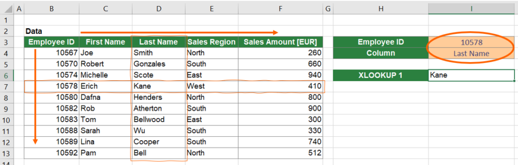
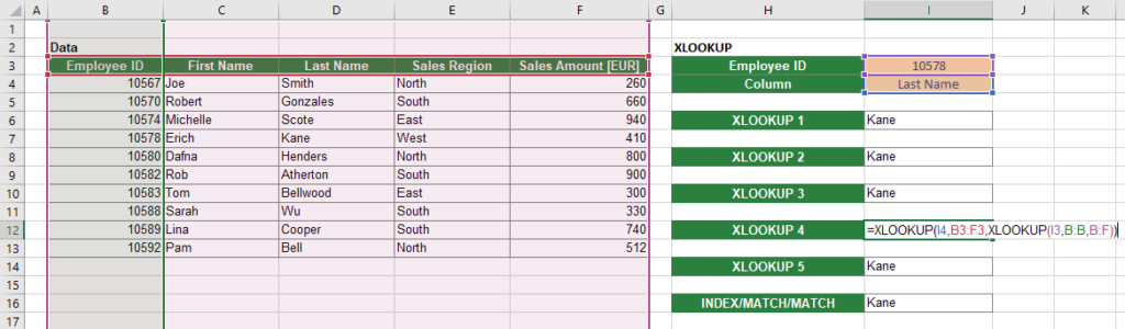
Our example: Based on the input in cells I3 and I4, we want to return the correct value from the table on the left-hand side. So, with the current inputs, we search for the Employee ID “10578” in column B and for “Last Name” in the rows. The return value in this example should be the Last Name of employee 10578 which is “Kane”.
For 2D XLOOKUPs there are multiple versions leading to the correct result. It’s all about using matching cell ranges in the arguments.
2D XLOOKUP step-by-step
The approach is to use a XLOOKUP to return a range of cells containing with all the last names. From this, we pick the correct one, belonging to ID 10578.
- We search for the name from top to the bottom. Because the vertical search value is given in cell I3, the XLOOKUP function starts with
=XLOOKUP(I3. - We search in the cell range B3 to B13 for the ID:
=XLOOKUP(I3,B3:B13.
Now we continue with the second XLOOKUP:
=XLOOKUP(I3,B3:B13,XLOOKUP( - The second / inner XLOOKUP searches for “Last Name”, provided in cell I4. That means, the second XLOOKUP starts with I4:
=XLOOKUP(I3,B3:B13,XLOOKUP(I4, - Next, we put in the search area, which is the cell range B3 to F3 (the headings of the columns).
=XLOOKUP(I3,B3:B13,XLOOKUP(I4,B3:F3, - Now comes the trick: We want the second XLOOKUP not to return a single value, but rather a range of cell, all the last names. That’s why we refer to the whole table, which is B3 to F13.
=XLOOKUP(I3,B3:B13,XLOOKUP(I4,B3:F3,B3:F13))
(Don’t forget the two closing brackets at the end.)
That’s it already. The 2D XLOOKUP looks like this:
=XLOOKUP(I3,B3:B13,XLOOKUP(I4,B3:F3,B3:F13))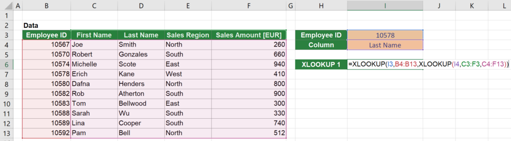
Please note: In the download (see below), this solution is labeled “XLOOKUP 1”. You can also find 4 more versions and the respective INDEX/MATCH/MATCH function.
What happens in this 2D XLOOKUP?
Before we continue with the next example, let’s inspect what happens here. If we just type the inner XLOOKUP, we receive the following result.
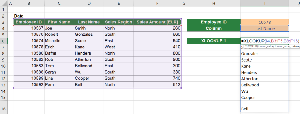
The return value is spilled down over many cells. As you can see, it returns all last names.
This is special about the XLOOKUP function: It can not only return a single value, but also a range of cells. We use this to wrap around the next XLOOKUP, to search and return the correct name from it.
Second example for 2D XLOOKUPs
Our second example has a minor to our first one: We insert the 2D XLOOKUPs to a complete column. However, the basic structure and the arguments of the XLOOKUP functions remain more or less the same.
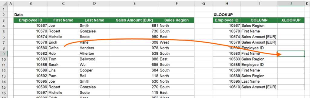
The goal: Fill in the correct values in column J by using two nested XLOOKUP functions on the Data table. For example, cell J9 should say “Dafna” because it’s the “First Name” of employee with ID “10580” (indicated by the orange arrow). In the following, we will use this cell (J9) to set up the 2D XLOOKUP function.
The second 2D XLOOKUP step-by-step again
So, how do we start? Actually, it’s the same as before, applying the structure as described above.
- The vertical search value now is the employee ID, given in cell H9.
=XLOOKUP(H9, - Because we search for the employee ID in column B, specifically range B3:B100003, the second argument is:
=XLOOKUP(H9,$B$3:$B$100003, - The horizontal search value is the column name. Setting up the second, inner XLOOKUP function in cell J9, it would be I9.
The inner function looks like this now:
=XLOOKUP(H9,$B$3:$B$100003,XLOOKUP(I9, - The second argument of the inner function is the column names. Adding a reference to the header row to the XLOOKUP function leads to:
=XLOOKUP(H9,$B$3:$B$100003,XLOOKUP(I9,$B$3:$F$3,
Because when we copy the function later we want to keep this reference the same, we add the $-signs. The cell reference is now a “absolute reference“. - As the third argument of the inner XLOOKUP function, just refer to the entire table. In this case, it’s $B$3:$F$100003:
=XLOOKUP(H9,$B$3:$B$100003,XLOOKUP(I9,$B$3:$F$3,$B$3:$F$100003)
Also here, fixate the cell references using the $-sign so that they won’t adapt when copying the function later-on.
=XLOOKUP(H9,$B$3:$B$100003,XLOOKUP(I9,$B$3:$F$3,$B$3:$F$100003))Variations for 2D XLOOKUPs
The 2D XLOOKUP function is quite open for variations.
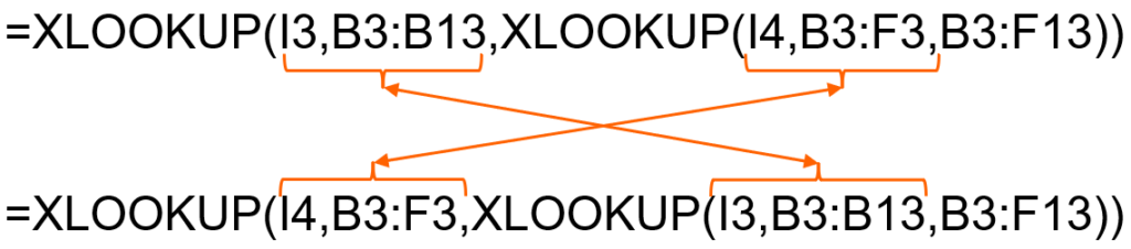
The sequence of the two XLOOKUPs doesn’t matter in 2D XLOOKUPs
Don’t understand me wrong, of course the sequence of arguments matters in general. But you can switch the meaning of the inner and outer XLOOKUP. So, the inner XLOOKUP doesn’t necessarily have to return a vertical range of cells. It could also return a horizontal range.
Let’s illustrate that a little bit. The function of our first example was:
=XLOOKUP(I3,B3:B13,XLOOKUP(I4,B3:F3,B3:F13))You can change it to:
=XLOOKUP(I4,C3:F3,XLOOKUP(I3,B4:B13,C4:F13))Or easier to read:
You can use complete column or row references – but not both at the same time
Often it makes sense not only to refer to the exact same ranges. For example, when you permanently add data. In such case, it’s helpful to refer to entire columns or row.
Also within the 2D XLOOKUP function, you can refer to entire columns as shown in the screenshot below.
You can also refer to entire columns. But you can’t refer to both, entire rows and columns at the same time.
Advantages and disadvantages of a 2D XLOOKUP compared to INDEX/MATCH/MATCH
INDEX/MATCH/MATCH is the classic approach for a 2D lookup in Excel. Two MATCH functions are nested into the INDEX function. Before we explore the advantages and disadvantages, let’s start with a similarity: Both functions are not easy to set up for beginners. But after some trial and error – and a guide like this 😉 – both should be manageable. Plus, they require the same basic inputs just in a different structure.
Advantages of 2D XLOOKUPs vs. INDEX/MATCH/MATCH
- 2D XLOOKUPs need a fewer number of arguments (the MATCH functions need a “0” in the end) and one nested function less. So, it’s slightly less complex.
- The XLOOKUP version offers built-in advanced functions, such as a binary search to speed it up or the IFNA function.
Advantages of INDEX/MATCH/MATCH vs. 2D XLOOKUP
- XLOOKUP is only available for newer Excel versions. Coming with this, “old” Excel users are more familiar with INDEX/MATCH and INDEX/MATCH/MATCH
- XLOOKUP, when not using the binary search, has a slower calculation performance.
- INDEX/MATCH/MATCH can even be extended for a 3D-Lookup.
That said: For basic usage, they both work. So, please feel free to use either one – maybe it’s time now to try the new, 2D XLOOKUP?
Do you want to boost your productivity in Excel?
Get the Professor Excel ribbon!

Add more than 120 great features to Excel!
Download the examples for 2D XLOOKUPs
Please download the examples from this article here. They not only include the versions of 2D XLOOKUPs from in this article, but also more variation.
And even more: Besides the examples above, the download has an exercise sheet on which you can practice the 2D XLOOKUP. When you are done – or stuck – check the solution.
Thank you! Followed a few guides and had some trouble but this page helped me understand and get my formula to work. I had months going across rows 1 and categories on column A and wanted to lookup the result for each category, within a specific month. This helped!
Thanks for the feedback, that’s great to hear!
hi, i don’t understand. i am trying a 2-way (horizontal and vertical) XLOOKUP and it’s working when all data on the same sheet and format is simple. but when i try to create an Xlookup looking to a different sheet, albeit in the same file, even when making sure the format cell is the same, i get an #Value error. the part that puzzles me the most is that when i do the xloop for the horizontal part and vertical part separately, they both woth but when combined, it returns this error. any idea? thanks
It works, this is amazing.
Thanks,