Combine Text in Excel: 5 Easy Methods to Concatenate Cells!

Excel offers three distinct functions as well as a fourth way to combine multiple text cells into one cell. There are countless examples in which you might need this: Combine given- and family names or preparing primary keys for multi-conditional lookups. For example, in a VLOOKUP or INDEX/MATCH formula combination. In this article you learn five methods and in the end, you learn how to deal with a large range of cells.

Method 1: &-sign

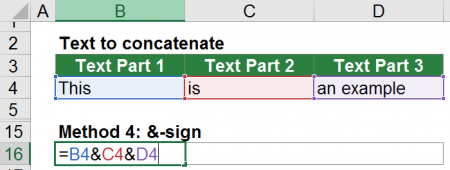
The easiest way is probably to just use the “&”-sign to combine values in Excel. This method has the same disadvantages like the CONCATENATE function from the method 4 below. It can only regard single cells and not ranges of cells. An advantage of this method is that it’s usually easier to follow up the calculation steps.

As you can see in the screenshot above, you can just refer to several cells and combine them with the &-sign. That’s it.

Method 2: CONCAT function

The CONCAT function has been introduced to Excel with the version 2016. It’s not available on previous versions of Excel. And that’s already the biggest disadvantage. Besides that, this function is very useful.

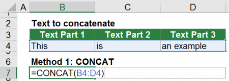
The CONCAT is the successor oft he CONCATENATE function and has at least one and at maximum 254 arguments. It can handle separate cells as well as cell ranges. It’s even possible to combine single cells with cell ranges, e.g. =CONCAT(B4,C4:D4) .

As you can see in the screenshot above, using the CONCAT function is very easy. Just refer to the cells you’d like to combine.

Method 3: Insert text to cell without any formula or function

You don’t want to use a formula or function but just add some text into existing cell? I have written a whole article about that.

The fastest way is to use Professor Excel Tools:

1. Select your original cells and click on the Insert Text button on the Professor Excel ribbon.
2. Choose, where (at the beginning or end of the existing text) you want to insert the additional text. You can further define, if you want to insert normal text, subscript or superscript.
3. Click on Start.

Click here to download Professor Excel Tools. For more information about the Excel add-in, please refer to this site.

Method 4: CONCATENATE function

Unlike the CONCAT function, CONCATENATE is available in older versions of Excel. Microsoft says within the help section of the CONCATENATE function, that the CONCATENATE is replaced by CONCAT. CONCATENATE is only kept in Excel in order to guarantee the compatibility to older versions on Excel and it’s recommended to use CONCAT instead.
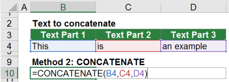
CONCATENATE works almost the same way like CONCAT with one major difference: It’s not possible to use ranges of cells as references. Only single cells can be combined. The maximum number of arguments and therefore single cell references is 255.

Method 5: TEXTJOIN function to combine cells

Since Excel 2016 there is another, advanced option to combine text in Excel. The function is called TEXTJOIN. Besides simply putting text together, the formula offers two advanced options:

1. You can define a separator between each cell you want to combine, for example a comma.
2. The formula provides the option to automatically skip blank (empty) cells.

The structure of the TEXTJOIN formula is shown in the figure above. The formula has at least three arguments.

1. Delimiter: The letter or word is added in-between and separates each cell input. A common delimiter is a comma.
2. Ignore empty: The second argument is either TRUE or FALSE. If set to TRUE or skipped, blank (empty) cells won’t be regarded. If set to FALSE, empty cells will also be regarded and separated by the delimiter.
3. The TEXTJOIN function requires at least one argument for the cells or text to be combined. This can be a cell range, a single cell or a value. It’s possible to use up to 252 references.

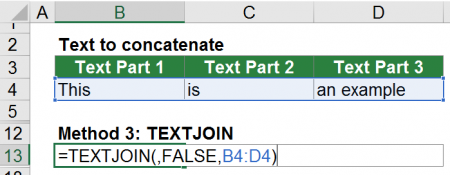
The screenshot of the example on the right-hand side shows an example for the TEXTJOIN formula. The first part is skipped which means that there is no delimiter. The second argument is set to FALSE so that blank cells aren’t ignored. Eventually the last argument refers to the cell range B4 to D4 which contains the cells to be combined. 

Example: Combine many cells in Excel

Let’s say, you want to combine 1,000 Excel cells into one cell. The good news: You can use all four methods to accomplish this, even in a simple manner. There is one restriction though: One Excel cell can’t contain more than 32,768 characters.

For combining 1,000 cells in Excel, you can use two basic approaches:

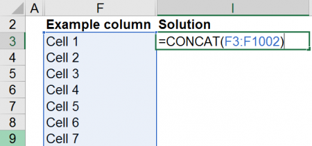
1. Use method 1 (CONCAT formula) or method 3 (TEXTJOIN formula) above which can regard cell ranges. The solution using the CONCAT formula is shown in Figure 66. As noted before, the only requirement of this method is that you have to use Excel version 2016.

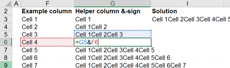
2. Insert a helper column (or row, depending on how your data is organized) which always combines the current cell with the previous combination of all cells so far. As you can see in the image on the right-hand side, the helper column (here in cell G6) combines cells G5 (which contains the previous combination) with the current cell F6. The solution in cell I3 only links to the last row in the helper column.

Download with all combine examples

All the examples above can be found in this example workbook.

Please click here and the download starts immediately.

Image by anncapictures from Pixabay