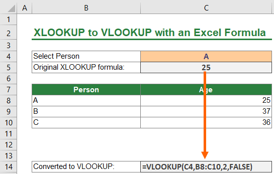
The new XLOOKUP formula in Excel is great. It’s very powerful and solves many problems the iconic VLOOKUP (or HLOOKUP) formula cannot do. But there is one problem: It’s only available in the newest Excel versions. Older versions – which are still around a lot – can’t use them. In this article we explore 4 ways to convert XLOOKUP to VLOOKUP.
Overview of the big XLOOKUP series
- Part 1: Basics of XLOOKUP
- Part 2: Advanced XLOOKUP – “If not found”, “Wildcard” and “Classification”
- Part 3: 2D-XLOOKUPs
- Part 4: Let’s talk about performance of XLOOKUP
- Part 5: Convert XLOOKUP to VLOOKUP (this article)
Prerequisites and disclaimer
Before we start, we unfortunately have to go through some requirements of your XLOOKUP formula as well as a disclaimer.
- These methods only work for a simple version of the XLOOKUP function. That means that only the first three arguments are used. The last three arguments (which are optional) are not used.
- Also, no nested functions: the formula is not wrapped in any other formula or contains other formulas within its arguments. If you have a formula combination, you’ll probably have to dig deeper – although methods 1 and 2 below might still help you.
- Please save backups of your work before you start. Especially the VBA macro (method 4 below) might cause irreversible changes to your formulas.
Method 1: Manually convert XLOOKUP to VLOOKUP
The first method – as usual – is the manual way. Often this is the fastest. Please follow these steps:
- Replace the X in XLOOKUP with V for VLOOKUP.
- The first argument stays the same.
- The second argument in the VLOOKUP formula is a comination of the 2nd and 3rd argument of XLOOKUP.
- Take a look at the 2nd and 3rd argument of XLOOKUP. How many column are there in-between. So if you are counting let’s say from column D to G, the “distance” of these two columns would be 3 columns (columns E, F and G). For VLOOKUP, you still have to add 1.
- The last argument is “FALSE”.

Example: Let’s take a look at an example. Your XLOOKUP formula looks like this: =XLOOKUP(A1,B1:B10,C1:C10)

- Replace XLOOKUP by VLOOKUP: =VLOOKUP(A1,B1:B10,C1:C10)
- The first argument (A1) remains the same: =VLOOKUP(A1,).
- Combine the first part of the second argument (B1 of the argument B1:10) and combine it with the last part of the 3rd argument: =VLOOKUP(A1,B1:C10,).
- Count the number of columns between the second and third argument of the original XLOOKUP formula and add 1: B to C has the distance of 1 column; after adding one, 2 is the third argument. =VLOOKUP(A1,B1:C10,2).
- Last argument is “FALSE”: =VLOOKUP(A1,B1:C10,2,FALSE).
Method 2: Transform cells containing XLOOKUP to hard values
The second method – transforming formula cells to “hard” values – can be achieved in two ways. Manually by copying and pasting respective cells or “automatically” by using a slightly smarter VBA macro.
Copy & Paste
Select the cell are range of cells containing XLOOKUP formulas. You can use the search function to identify these cells. As a side note: Please don’t copy and paste non-coherent cells.
Now copy these cells by pressing Ctrl + C on the keyboard. Next paste these cells with “Paste special”: Hold Ctrl + Alt on the keyboard and press V. Select “Values” and click on “OK”.
Please refer to this article for more information about pasting formulas as values only.
VBA Macro
You don’t like to convert XLOOKUP formula cells to values manually but rather use a VBA macro? Please feel free to use the following macro. It converts all cells that have formulas and have the string XLOOKUP within them to values. Of course the warning: Please be careful, the XLOOKUP and therefore your workbook does not work as before. And there is no undo function.
Add the code to your Excel file (please refer to this article for more detailled description of how to add VBA code to your Excel file):
- Open the VBA editor (Alt + F11 on the keyboard).
- Insert a new module.
- Paste the code below and place the cursor within the code.
- Press start.
Sub Convert_XLOOKUP_to_Values()
Dim formula_text As String
For Each cell In ActiveSheet.UsedRange

    If cell.HasFormula = True Then
        formula_text = cell.Formula

        If InStr(1, formula_text, "XLOOKUP") > 0 Then
            cell.Select
            cell.Copy
            cell.PasteSpecial xlPasteValues
        End If
    End If
Next

Application.CutCopyMode = False
End Sub
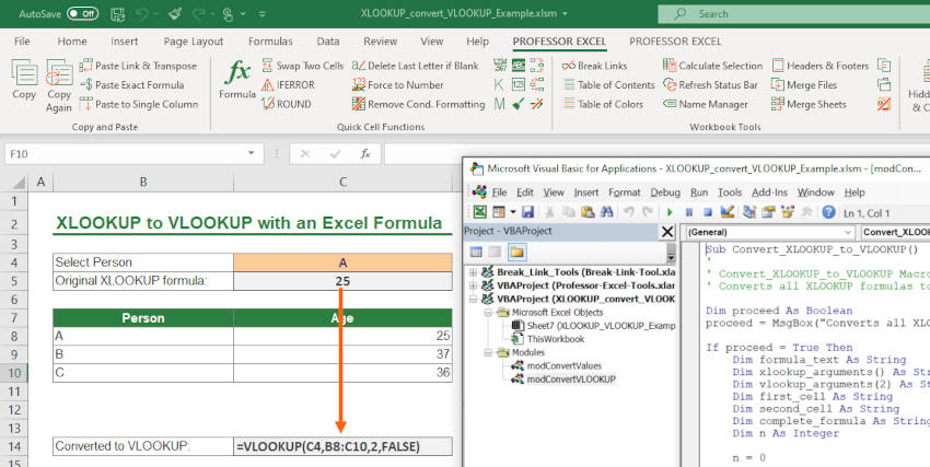
Recommendation: Please check the example workbook. In the download workbook, please find the VBA macro in the module “modConvertValues”.
Method 3: Use an Excel formula to convert XLOOKUP to VLOOKUP or HLOOKUP
You don’t like VBA / macros? This methods works without any VBA code and with only minimal manual work.

The idea: You copy and paste a long formula (see below) into your sheet. Then you just do a tiny modification (by search & replace). The output of the formula is a VLOOKUP formula, based on your input XLOOKUP formula.
So let’s assume that your XLOOKUP formula is located in cells B3.
- Copy the Excel formula (below) into an empty, unused cell. In the picture above, it was copied into cell C14.
- Replace all occurrences of “A1” by your XLOOKUP formula cell, B5. Fastest would be the Find & Replace function (press Ctrl + H on the keyboard to open the dialogue).
The output of the formula is the converted VLOOKUP formula. - Copy and paste it (as values) into cell B5. Press one time F2 and Enter in order to eventually convert the text to formula.
="=VLOOKUP("&MID(FORMULATEXT(A1),FIND("(",FORMULATEXT(A1))+1,FIND(",",FORMULATEXT(A1))-FIND("(",FORMULATEXT(A1))-1)&","&MID(FORMULATEXT(A1),FIND(",",FORMULATEXT(A1))+1,FIND(":",FORMULATEXT(A1))-FIND(",",FORMULATEXT(A1))-1)&":"&MID(FORMULATEXT(A1),MATCH(2,1/(MID(FORMULATEXT(A1),SEQUENCE(LEN(FORMULATEXT(A1))),1)=":"))+1,LEN(FORMULATEXT(A1))-MATCH(2,1/(MID(FORMULATEXT(A1),SEQUENCE(LEN(FORMULATEXT(A1))),1)=":"))-1)&","&COLUMN(INDIRECT(MID(FORMULATEXT(A1),MATCH(2,1/(MID(FORMULATEXT(A1),SEQUENCE(LEN(FORMULATEXT(A1))),1)=":"))+1,LEN(FORMULATEXT(A1))-MATCH(2,1/(MID(FORMULATEXT(A1),SEQUENCE(LEN(FORMULATEXT(A1))),1)=":"))-1)&"1"))-COLUMN(INDIRECT(MID(FORMULATEXT(A1),FIND(",",FORMULATEXT(A1))+1,FIND(":",FORMULATEXT(A1))-FIND(",",FORMULATEXT(A1))-1)&"1"))+1&",FALSE)"
Recommendation: Check the example in the workbook. In the the download workbook, the Excel formula is located in cell C14 of the only worksheet.
Method 4: Convert all XLOOKUP formulas to VLOOKUP with this VBA macro
The last method is also the most complex one: Convert all XLOOKUP formulas in your current worksheet to VLOOKUP with a VBA macro.
One more time the warning:
- Please be careful, the XLOOKUP and therefore your workbook does not work as before.
- There is no undo function.
- Also this VBA macro only works for the simple version of XLOOKUP formula, having only 3 arguments and the lookup works from left to right (this article has more information about VLOOKUPs to the left).
Add the code to your Excel file (please refer to this article for more detailled description of how to add VBA code to your Excel file):
- Open the VBA editor (Alt + F11 on the keyboard).
- Insert a new module.
- Paste the code below and place the cursor within the code.
- Press start.
Sub Convert_XLOOKUP_to_VLOOKUP()
'
' Convert_XLOOKUP_to_VLOOKUP Macro
' Converts all XLOOKUP formulas to VLOOKUP. Careful: Only works with simple XLOOKUP formulas. Please save a backup first - undo not possible.

Dim proceed As Boolean
proceed = MsgBox("Converts all XLOOKUP formulas to VLOOKUP. Careful: Only works with simple XLOOKUP formulas. Please save a backup first - undo not possible.", vbOKCancel, "Careful!")

If proceed = True Then
    Dim formula_text As String
    Dim xlookup_arguments() As String
    Dim vlookup_arguments(2) As String
    Dim first_cell As String
    Dim second_cell As String
    Dim complete_formula As String
    Dim n As Integer

    n = 0

    'Go trough all cells in used range
    For Each cell In ActiveSheet.UsedRange.Cells

        'Only regard formula cells
        If cell.HasFormula = True Then
            formula_text = cell.Formula

            'Only use formulas starting with XLOOKUP
            If Left(formula_text, 9) = "=XLOOKUP(" Or Left(formula_text, 1) = "=+XLOOKUP(" Then

                'Split the formula into its arguments
                xlookup_arguments = splitString(CStr(formula_text))

                'Write new arguments one by one
                vlookup_arguments(0) = xlookup_arguments(0)
                first_cell = Split(xlookup_arguments(1), ":")(0)
                second_cell = Split(xlookup_arguments(2), ":")(1)
                vlookup_arguments(1) = first_cell & ":" & second_cell

                'Handle difference of column cell range ("A:B") and other cell range ("A1:B5")
                If string_has_number(CStr(first_cell)) = True Then
                    number_of_columns = Range(second_cell).Column - Range(first_cell).Column
                Else
                    number_of_columns = Range(second_cell & "1").Column - Range(first_cell & "1").Column
                End If

                'add one for VLOOKUP distance because VLOOKUP starts counting with the first column/cells
                vlookup_arguments(2) = number_of_columns + 1

                complete_formula = "=VLOOKUP(" & vlookup_arguments(0) & "," & vlookup_arguments(1) & "," & vlookup_arguments(2) & ",FALSE)"

                cell.Formula = complete_formula
                n = n + 1
            End If

        End If
    Next

    Dim confirm As Boolean
    If n = 0 Then
        confirm = MsgBox("No XLOOKUP formula converted", vbExclamation, "Done")
    Else
        confirm = MsgBox(n & " XLOOKUP formulas to VLOOKUP converted. Please check them and if necessary revert back to your previously saved backup file.", vbExclamation, "Done")
    End If
End If


End Sub


Function splitString(formula_text As String)
    Dim Result() As String
    Dim DisplayText As String
    Dim arguments As String
    arguments = Replace(formula_text, "=XLOOKUP(", "")
    arguments = Replace(arguments, "=+XLOOKUP(", "")

    Result = Split(arguments, ",")
    Result(2) = Replace(Result(2), ")", "")

    splitString = Result
End Function

Function string_has_number(first_cell As String) As Boolean
    Dim i As Integer

    For i = 1 To Len(first_cell)
        If IsNumeric(Mid(first_cell, i, 1)) Then
            string_has_number = True
            Exit Function
        End If
    Next

End Function
Recommendation: In the download workbook, please find the VBA macro in the module “modConvertVLOOKUP”.
Download

Please feel free to download all examples, including all VBA macros in this article, from this link.


