VLOOKUP to the Left in Excel. Yes, It’s Possible!

The VLOOKUP formula in its base version only works from left to right. The search column must be located on the left-hand side of the return column. What if your data doesn’t have such structure? There is a way for using the VLOOKUP to the left but it requires an array form of the formula. It’s often worth considering alternative formulas though. Here is everything you should know.

Before we start with the VLOOKUP to the left: Yes, it’s possible. But in most cases not recommended. Take a look at the new XLOOKUP function. Or INDEX/MATCH. They usually work much better. That said: Let’s get started!

Alternatives to the VLOOKUP formula

The VLOOKUP formula can be used for returning a value on the left of a search value. But you have to use it in the array form. Because using the VLOOKUP formula as an array formula comes with several disadvantages, please consider two different approaches if your search column is on the right-hand side of the return column.

1. Use a different formula. INDEX/MATCH works very well because you specifically select both the search and the return column. This method has some advantages towards the following methods: It’s fast, slightly faster than a “normal” VLOOKUP and significantly faster than a VLOOKUP in the array form. Also, setting up the INDEX/MATCH formula is usually easier than using the VLOOKUP formula in the array form. Another advantage is that you don’t have to touch the original data (e.g. add columns or change the sequence of columns).
   If your return value is numeric (including dates) you could use the SUMIFS formula as well. But please make sure that your search value only comes up once in your data. Otherwise the SUMIFS formula returns the sum of all the occurrences of the search value.
2. Re-organize your data. Either change the sequence of columns or add a new column on the right-hand side of your existing data, linking to the return value.

VLOOKUP formula in the array form

Structure of VLOOKUP to the left

Like in the previous article—multi-condition lookups—the trick is to create a virtual table (an array) using the CHOOSE formula within the VLOOKUP formula. In this virtual table, you change the structure of the input data so that the search value is located on the left-hand side of the return value.

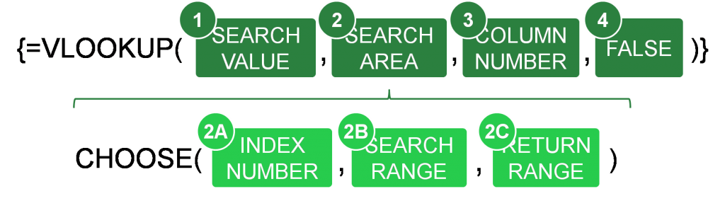
The structure of the VLOOKUP formula is shown in image on the right-hand side.

1. The SEARCH VALUE is as always in the VLOOKUP formula the value you are looking for.
2. As mentioned before, the CHOOSE formula creates a two-dimensional array. The first column of this CHOOSE formula contains the search column and the second range has the return value.
   1. The INDEX number of the CHOOSE formula is always {1,2}.
   2. The search column.
   3. The last part of the CHOOSE formula is the return column or return range.
3. The column number is always 2 because the you want to return the second column from the virtual table of the CHOOSE formula.
4. Eventually the last argument of the VLOOKUP formula is “FALSE”.

As usual for array formulas, press Ctrl + Shift + Enter after you finished typing. The curly brackets are added automatically that way.

Example for the VLOOKUP to the LEFT

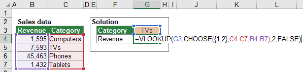
Say you have sales data in the cell range B4 to C7 like shown in the screenshot on the right-hand side. The revenue is given in the cell range B4 to B7 and the category in C4 to C7. The task is to return the revenue depending on the selection of the category.

That means you have to following input values:

• SEARCH VALUE: The search value is the selection of category for which you want to return the revenue. It is located in cell G4.
• INDEX NUMBER: Always {1,2} for VLOOKUP to the left.
• SEARCH RANGE: You search within the cell range C4 to C7 for the category.
• RETURN RANGE: Because you want to return the revenue, the return range is B4 to B7.
• COLUMN NUMBER: As mentioned before, the column number is 2 because you want to return the second column of the virtual CHOOSE table.

Assembling all these inputs you will have the following formula for a VLOOKUP to the left.

{=VLOOKUP(G3,CHOOSE({1,2},C4:C7,B4:B7),2,FALSE)}

Again, don’t forget to press Ctrl + Shift + Enter instead of just Enter on the keyboard after you finish to type the formula.

HLOOKUP bottom-up

Actually, I’ve only added this section for the sake of completeness. In most cases (well, I can’t think of a case you should use the HLOOKUP formula bottom-up) I’d recommend using INDEX/MATCH in a horizontal way instead.

HLOOKUP works top-down. But like the VLOOKUP formula before it can be used to work bottom-up. The structure of the HLOOKUP formula in the array form is very similar to VLOOKUP in the previous section. There is one difference, though: You have to add the TRANSPOSE formula within and around the CHOOSE formula in order to convert the horizontal cell ranges to vertical cell ranges. Again, there are usually easier options for achieving an HLOOKUP from bottom to the top.

The structure of the HLOOKUP formula is shown in the screenshot on the right-hand side. The numbered arguments in this screenshot are the same like in the VLOOKUP formula to the left above.

An example for the bottom-up HLOOKUP is shown in image below. Like before you want to return the revenue from the cell range C3 to F3 based on the selection of the category in cell range C4 to F4.

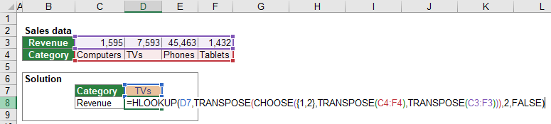
Assembling the argument in Figure 102 leads to the following formula.

{=HLOOKUP(D7,TRANSPOSE(CHOOSE({1,2},TRANSPOSE(C4:F4),TRANSPOSE(C3:F3))),2,FALSE)}

Please note:

• Array formulas in general need longer calculation times than their “normal” counterpart formulas. It’s not recommended using them in a large scale. Also try to refer to the exact cell range instead of entire columns or rows.
• Please keep in mind when using such array formula solution that array formulas are more difficult to apply, to debug and to understand for other Excel users than normal formulas.

Download

Please feel free to download an Excel workbook with all the examples from this article. Just click this link and the download starts immediately.