
There are many cases in which you want to conduct a lookup with several search criteria. As of now only the SUMIFS formula allows a multi-condition lookup. Unfortunately, SUMIFS only works for numeric values (including dates) as the return value. If you want to return text, there is no direct method.
The good news: Both major lookup formulas besides SUMIFS (VLOOKUP, and INDEX/MATCH) allow workarounds. The easiest way is usually an additional helper column. But also array formulas can be used for multi-condition lookups – even without helper columns.
The example for all methods of multi-condition lookups
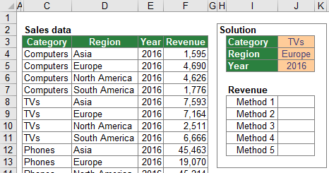
In this article, you explore five methods for multi-condition lookups. All methods will be introduced using the same example like shown in the screenshot on the right-hand side.
You have a table containing sales data with the columns “Category” (column C, e.g. “Computers”, “TVs”), “Region” (column D, e.g. “Asia”, “Europe”) as well as the “Year” (column E, e.g. “2016”). The return value (here: “Revenue”) is provided for each combination of category, region and year in column F. The cells J3 to J5 contain selection fields for each of the columns. For example, you want to return the revenues of TVs in Europe in the year 2016. The return value should be shown in the cell J8 to J12, depending on the method in this chapter.
Method 1: VLOOKUP and helper column
As mentioned before, there is no direct way to conduct a lookup with several conditions using VLOOKUP formula. But there is a simple workaround: Insert a new “primary key” column. To achieve this, concatenate the different search values in a new (leftmost) column.
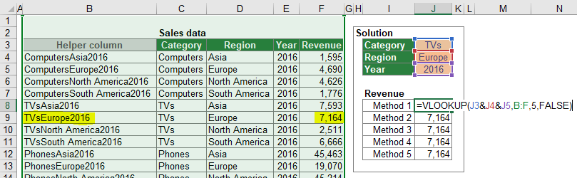
The first step is to insert the new column B with the new primary key. You can easily concatenate the values from the columns C, D and E by using the “&” sign. The formula in B4 is =C4&D4&E4 .
In the second step, you set up the VLOOKUP formula. The search term is not one single search criteria. Instead, you search for the combination of “Category”, “Region” and “YEAR”. The search range starts now with column B which contains the new primary key. The return value is located in column F so that the column number is 5. As usual the last argument of the VLOOKUP formula is “FALSE” because you search for the exact search phrase. The complete VLOOKUP formula is: =VLOOKUP(J3&J4&J5,B:F,5,FALSE)
Please note the following comments.
- Keep in mind that the search column must be located on the left-hand side of the return column.
- Please note that if you use a helper column for a lookup with multiple search criteria, please make sure that the new primary key is actually unique and doesn’t exist multiple times. For example, say you have the two data sets “value1”&”22” and “value12”&”2.” If they were combined in a new primary key, then both would say “value122.” Separating both cells with an additional character could help—for example, by adding a space character or any other separator—but that is not necessarily a safe solution.
- In terms of calculation performance, Excel can handle large cell ranges quite well. In the example above, the search range refers to the whole columns B:F.
Method 2: VLOOKUP without helper column
The first method in the previous pages of the multi-condition VLOOKUP required an additional helper column. The method in this section is a little bit more complex but has the advantage that it doesn’t need an additional column.

Because the underlying formula of this method is still VLOOKUP, the arguments are more or less the same. The following numbers correspond to the numbers in the screenshot on the right-hand side, which shows the structure of the VLOOKUP/array formula.
- The SEARCH VALUE is the combination of the three conditions. In this case the search values are given in cells J3 to J5 so that this argument is J3&J4&J5.
- The idea is that the CHOOSE formula creates a two-dimensional array. You can imagine at as a table with two columns. The first column contains the search phrase, in this case the combination of all three search criteria (e.g. “ComputersAsia2016”). The second range has the revenue.
- The INDEX number of the CHOOSE formula is always {1,2}.
- The first search column. You combine it using the &-sign with …
- …the second search column…
- …and the third search column. You can also add more search columns here if you have more conditions.
- The last part of the CHOOSE formula is the return column or return range.
- The column number is always 2 because the you want to return the second column from the virtual table of the CHOOSE formula.
- Eventually the last argument of the VLOOKUP formula is “FALSE”.
Applying this structure to the example in this chapter you get the following formula.
{=VLOOKUP(J3&J4&J5,CHOOSE({1,2},C4:C51&D4:D51&E4:E51,F4:F51),2,FALSE)}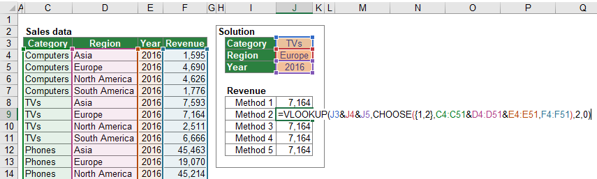
Please note the following comments:
- Don’t forget to press Ctrl + Shift + Enter after typing the formula because this is an array formula. If you just press Enter on the keyboard, the formula will return a wrong result instead of an error message.
- Please try to minimize the cell ranges within the CHOOSE formula. Don’t use complete columns. As mentioned before, in “normal” formulas, Excel can handle large cell references quite well. In array formulas using complete rows or columns will lead to long calculation times.
Method 3: INDEX/MATCH and helper column
The third method for a multi-conditional lookup uses the INDEX/MATCH formula and an additional helper column. It pretty similar to method 1 before because the helper column works the same way. Besides that, it’s based on a conventional INDEX/MATCH formula.
The idea of this method is to create a helper column in which you concatenate all search criteria. Unlike the helper column of method 1 (VLOOKUP and helper column), the helper column can be located anywhere on your worksheet. It doesn’t have to be on the left-hand side of the return column.
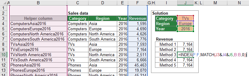
The formula in the helper column (here: cell B4) is =C4&D4&E4 .
You apply a “normal” INDEX/MATCH formula with the only difference that you search for the combination of criteria within the MATCH part of the formula. The formula (here in cell J10) is =INDEX(F:F,MATCH(J3&J4&J5,B:B,0)) .
Do you want to boost your productivity in Excel?
Get the Professor Excel ribbon!

Add more than 120 great features to Excel!
Method 4: INDEX/MATCH without helper column
A helper column always means additional work and in some cases, you want to leave the raw data untouched. The INDEX/MATCH formula combination can also be used without inserting a helper column. Like the method 2 before, the INDEX/MATCH formula is used like an array formula.

The structure of the multi-condition INDEX/MATCH formula is shown in the screenshot on the right-hand side. The following numbers relate to this figure.
- The cell array refers to the return cell range. In the example of this chapter it’s the revenue given in the column F. In order to save some calculation time it’s recommended to use the exact cell range instead of entire columns.
- The first argument of the MATCH formula is the lookup value. The multiple search values are concatenated to one search term.
- The lookup array combines the multiple search ranges with the & sign. It’s possible to have more than just the three search ranges as shown in screenshot above.
- The last argument of the MATCH formula defines the match type. For the multi-conditional lookup it’s always 0 in order to achieve an exact match.
Applying this structure to the example of this chapter leads to the following formula.
{=INDEX(F4:F51,MATCH(J3&J4&J5,C4:C51&D4:D51&E4:E51,0))}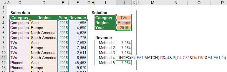
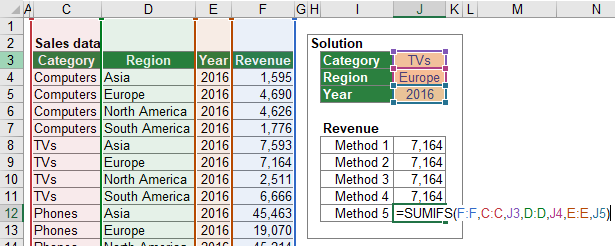
Method 5: SUMIFS
If your return value is a numeric value (including a date), you can use a SUMIFS formula without any additional modifications. The structure is described in detail starting in this article.
The example using the SUMIFS formula is shown in screenshot below.
Please note the following comments.
- You can only use the SUMIFS formula if each criteria combination only exists once in your data table. If Excel can find it multiple times, it will return the sum of all values that fulfill the search criteria combination.
- Most users would agree that entering the SUMIFS formula is easier than all the other previous methods. But SUMIFS is usually slower in terms of calculation speed than VLOOKUP and INDEX/MATCH. So, this method 5 is significantly slower than method 1 and method 3 before. Compared to methods 2 and 4 it’s not unambiguous which method is faster, depending mainly on the number of cells regarded in the search ranges.
Horizontal multi-conditional lookups
All methods described above work in a horizontally the same way with two exceptions.
- Instead of VLOOKUP you have to use HLOOKUP (regards methods 1 and 2).
- The HLOOKUP formula in method 2 (the array version) requires additional TRANSPOSE formulas.
All examples are also included horizontally in the download file below.
Download

Please feel free to download an Excel workbook with all the examples from this article. Just click this link and the download starts immediately.