VLOOKUP in Excel: All You Need to Know About the Powerful Function!

One of the most popular formulas in Excel is the VLOOKUP formula. Many lookup approaches are based on the VLOOKUP formula. Mastering it is crucial for any of the following chapters and methods. Unfortunately, VLOOKUP is not as easy to use as a SUM or COUNT. In this article, you learn how to use VLOOKUP, what to keep in mind and some more advices about VLOOKUP.

What do you need the VLOOKUP formula for?

The description text in Excel summarises it quite well:

Looks for a value in the leftmost column of a table, and then returns a value in the same row from a column you specify.

That means you got a table with data and you are searching for an item in the leftmost column. Once you’ve found the item, VLOOKUP will look into the same row and return a value in another column on the right hand side.

At this point it’s already important to note one of the major restrictions: VLOOKUP can only return values on the right-hand side of the search column. There is no exception to this rule. We will later come back to this restriction.

Info: The V in VLOOKUP stands for vertical. The corresponding formula for horizontal lookups is called HLOOKUP.

Structure of VLOOKUP

The VLOOKUP has four parts, of which three need to be defined. The fourth part is usually just “FALSÉ”, so we can omit this part for now. Let’s have a look at VLOOKUP step by step.

1. The first part contains the lookup value – the value you are searching for.
2. The second part defines the area you search in. Important: This area must include both columns:
   1. The search column in which you want to find your search value. This must be the leftmost column.
   2. The return value. So please make sure, your search area is large enough.
3. Now you have to count: Starting from your search column, you count the column until your return value column.
4. The fourth part is (for now) always “FALSE”.

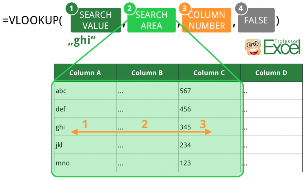
Let’s fill the definitions above with a simplified example. You want to search for “ghi” and get the number from column 3 returned.

1. As you search for “ghi” the first part is “ghi”.
2. A little bit more difficult: The search area. The area must include the search column and the return column. In our case that’s column 1 to column 3.
3. In which column is your return value? It’s the third column (counting from the search column). So you just fill in 3.
4. The fourth part is “FALSE”.

The complete formula looks like this: =VLOOKUP(“ghi”,A:C,3,FALSE)

Example for the VLOOKUP formula

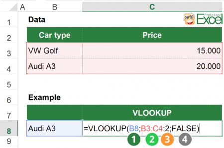
The picture on the right-hand side shows a simple usage of the VLOOKUP. The image shows a simple usage of the VLOOKUP. It searches for the value from cell B8 (“Audi A3) within the table above and returns the price from column C.

1. First part: The lookup value you search for. In this case, it refers to cell B8. Cell B8 has the value “Audi A3” so that means you search for “Audi A3”.
2. Second part: The cell range, in which you want to search in. In this example, it’s the table located above in the cells B3 to C4. Excel searches in the leftmost column of this cell range. Besides the search column, the column with the return value must also be included in this range.
3. Third part: The number of the column, which you want to be returned. So once Excel found “Audi A3” in the cell range B3 to B4, it returns the value from 2 columns on the right-hand side. Please keep in mind that the search column (here: B) counts as the first column. That means that the value from column C (the price) will be returned.
4. Fourth part: One optional value, which you can always be considered to be “FALSE” (it determines if you want to search for the exact value).

The complete formula is =VLOOKUP(B8,B3:C4,2,FALSE)

HLOOKUP works the same way as the VLOOKUP with the only difference, that the ranges are transposed: Instead of in a column, the HLOOKUP searches in a row (HLOOKUP = horizontal lookup; VLOOKUP = vertical lookup).

---

Do you want to boost your productivity in Excel?

Get the Professor Excel ribbon!

Learn more

Download Free Trial

Add more than 120 great features to Excel!

---

What if the last part is not “FALSE”?

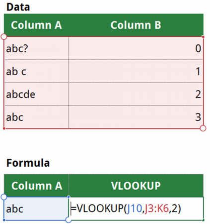
Before we’ve always said that the last part of the VLOOKUP formula must be “FALSE”. “FALSE” indicates in this case, that you want to search for the exact lookup value. If you search for “abc” you don’t accept “ab c” (with a space character). If you set it to “TRUE” or leave it blank, Excel will also return the “closest match”. The problem: You can’t be sure, if your value was exactly found or if Excel “thinks” that another value is a close match. Before we’ve always said that the last part of the VLOOKUP formula must be “FALSE”. “FALSE” indicates in this case, that you want to search for the exact lookup value. If you search for “abc” you don’t accept “ab c” (with a space character). If you set it to “TRUE” or leave it blank, Excel will also return the “closest match”. The problem: You can’t be sure, if your value was exactly found or if Excel “thinks” that another value is a close match. In the example above (you search for the closest match of “abc”), Excel considers “ab c” (with a space character) as a close match. It returns “1” from column B. In almost every case, you want to avoid such uncertainty: So please remember that the last part of the VLOOKUP formula is “FALSE”.

How to deal with the restriction that the return column must be right?

Oftentimes, the return value is located on the left side of your search value. Unfortunately, Excel doesn’t allow such case: You must use a workaround. There are basically four options.

1. Change the sequence of the columns in the lookup table. For example, move the column with the search value to the left side or the return column to the right side.
2. Alternatively, duplicate the column of the return value on the right-hand side. You can either just copy and paste it or create a link to the original value.
3. The third option is not using the VLOOKUP formula. The alternatives are SUMIFS or the combination of INDEX/ MATCH and the new XLOOKUP function.
4. Conduct a VLOOKUP to the left. Please refer to this article for more information.

VLOOKUP error messages

There are basically three major (alleged) error messages, which actually tell you quite well how to improve your formula. You should check your formula, if you got one of the following return values:

• #REF: Usually, your lookup range is not large enough. Make sure, that both your search and return column are within this range.
• #N/A: The value you are searching for is not available in your data. You could try searching it manually.
• #NAME: Check, if you misspelled “VLOOKUP”.
• 0: This is probably not an error message, but could be the real return value. For example, when your return cell is left blank, a “0” will be shown as the return value of the VLOOKUP.

If the above hints don’t help or there is another error message (such as “#DIV/0!”), try searching for the value manually. Maybe there is already an error in your data.

Tips & tricks for the VLOOKUP function

VLOOKUP is powerful and probably one of the most used formulas besides sum and count. To improve the usage, it’s recommended trying the following tips and tricks:

• In the third part of the formula, you have to determine the search range. Often, you’d copy and paste the formula so that it makes sense (whenever possible) to select whole columns instead of only small ranges. That makes the formula more stable.
• Also keep in mind that VLOOKUP only returns the first search result. If your search value occurs several times in your data, only its first occurrence will be returned.
• If you want to search for a combination of different criteria, there is no direct way with the VLOOKUP. One workaround could be by generating a new “primary key”. Therefore, concatenate the different search values in a new (leftmost) column.
• There are usually alternative ways instead of using VLOOKUP. Please take a look at our article about when to use VLOOKUP, SUMIFS or INDEX/MATCH.