
You’ve probably heard of VLOOKUP which is a very popular and powerful formula in Excel. Far less known is the little brother: HLOOKUP. It basically works the same way as VLOOKUP with one difference: Instead of looking up values vertically, HLOOKUP works horizontally. In this article, you learn how to use HLOOKUP, what to keep in mind, possible error messages and some more advices about HLOOKUP.
Before we start with the HLOOKUP: Do you know XLOOKUP? It’s new in Excel and has some advantages towards HLOOKUP. That said: Let’s get started!
What do I need HLOOKUP for?

The description text in Excel summarizes it quite well:
Searches for a value in the top row of a table or an array of values, and then returns a value in the same column from a row you specify in the table or array.
That means you got a table with data and you are searching for an item in the top row. Once you’ve found the value, HLOOKUP will look below within the same column and return a value from another row below.
HLOOKUP works the same way as the VLOOKUP formula with the only difference, that the ranges are transposed: Instead of in a column, the HLOOKUP searches in a row (HLOOKUP = horizontal lookup; VLOOKUP = vertical lookup).
Structure of HLOOKUP
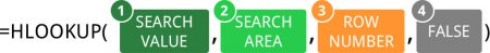
The HLOOKUP has four parts, of which three need to be defined. The fourth part is usually just “FALSE”, so we can omit this part for now. Let’s have a look at HLOOKUP step by step.
- The first part contains the lookup value – the value you are searching for.
- The second part defines the area you search in. Important: This area must include both rows:
- The search row in which you want to find your search value. This must be the top row.
- The return value. Please make sure, your search area is large enough.
- Now you have to count: Starting from your search row (that means the top row), you count the rows to your return value row.
- The fourth part is (for now) always “FALSE”.
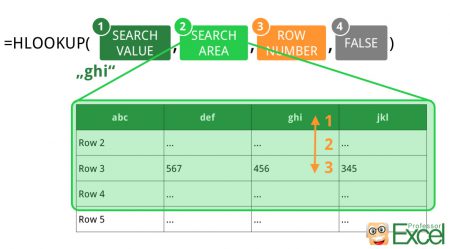
Let’s fill the definitions above with a simplified example. You want to search for “ghi” and get the number from row 3 returned.
- As you search for “ghi” the first part is “ghi”.
- A little bit more difficult: The search area. The area must include the search row and the return row. In our case that’s row 1 (the header row) to row 3.
- In which row is your return value located? It’s the third row (counting from the search row – the header row). So you just fill in 3.
- The fourth part is “FALSE”.
The complete formula might look something like this: =HLOOKUP(“ghi”,1:4,3,FALSE)
Do you want to boost your productivity in Excel?
Get the Professor Excel ribbon!

Add more than 120 great features to Excel!
Another example for the HLOOKUP formula
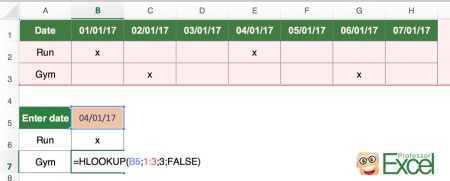
The image on the right hand side shows a simple usage of the HLOOKUP.
- First part: The lookup value you are searching for. In this case, it refers to cell B5. Cell B5 contains the date 04/01/17 so that means we are searching for date 4th of January 2017.
- Second part: The range, in which you want to search in. In our example, it’s the table on top. Excel searches in the topmost row of this range. Besides the search row, the row with the return value must also be included in this range.
- Third part: The number of the row, which you want to get returned. So once Excel found the date”04/01/17″ in the cells row 1, you have to define, which value you want it to get returned. In this example, you want to know if you go running or to the gym, which is written in column 2 or 3 respectively. As row 3 is the third row after 1 (which you search in), you have to write “3”. Keep in mind that the search row is always “1”.
- Fourth part: One optional value, which you can always consider to be “FALSE” (it determines if you want to search for the exact value).
The complete formula is =HLOOKUP(B5,1:3,3,FALSE)
One more example for the HLOOKUP formula

In this example we want to get tax rates from the table in the range C2 to H3. We want to search for the country in row 2 and return the tax rate from row 3.
Again, the HLOOKUP has four parts (example for cell D12):
- What do we search for? In cell D12 we want to get the tax rate for the “UK”. This value is given in cell C12. So the first part is “C12”.
- Where do we search? We search in row 2. As this range also has to cover the return row (in our case row 3) we could just write the rows 2:3. But in our example, we further specify column C to H, so that this part is “$C$2:$H$3”.
Please note: The dollar signs fix the range. If we copy and paste the formula, this range won’t change. - We want to return in value from the second row (the first row is the search row, row 2). That means the value for the third part of the HLOOKUP formula is “2”.
- As usual, the last part is “FALSE”.
The complete formula is =HLOOKUP(C12,$C$2:$H$3,2,FALSE)
HLOOKUP error messages
There are basically three major (alleged) error messages, which actually tell you quite well how to correct your formula. You should check your formula, if you got one of the following return values:
- #REF: Usually, your lookup range is not large enough. Make sure, that both your search and return rows are within this range.
- #N/A: The value you search for is not available in your data. You could try searching it manually.
- #NAME: Check, if you misspelled “HLOOKUP”.
- 0: This is probably not an error message, but could be the real return value. For example, when your return cell is left blank, a “0” will be shown as the return value of the HLOOKUP formula.
If the above hints don’t help or there is another error message (such as “#DIV/0!”), try searching for the value manually. Maybe there is already an error in your data.
Tips & tricks for the HLOOKUP formula
In order improve the usage of the HLOOKUP formula, it’s recommended trying the following tips and tricks:
- In the third part of the formula, you have to determine the search range. Often, you’d copy and paste the formula so that it makes sense (whenever possible) to select whole rows instead of only small ranges. That makes the formula more stable.
- Also keep in mind that HLOOKUP only returns the first search result. If your search value occurs several times in your data, only its first occurrence will be returned.
- If you want to search for a combination of different criteria, there is no direct way with the HLOOKUP. One workaround could be by generating a new “primary key”. Therefore, concatenate the different search values in a new (topmost) row.
- There are usually alternative ways instead of using HLOOKUP. Please take a look at our article about when to use VLOOKUP, SUMIFS or INDEX/MATCH.