Array Formulas in Excel: All You Need to Know

Array formulas are an advanced topic in Excel. Usually Excel users discover them when reaching the limits of – let’s call them – normal formulas, e.g. SUM, VLOOKUP, COUNT and so on. This article provides an introduction of array formulas in Excel.

Basics of array formulas

Microsoft writes about array formulas:

To become an Excel power user, you need to know how to use array formulas, which can perform calculations that you can’t do by using non-array formulas.

This article explains the basics of these formulas and provides examples.

Array formulas extend normal formulas. An array is a range of at least two or more cells. They are also referred to by “CSE” formulas which stands for Control, Shift, Enter. The reason is that after typing an array formula into an Excel cell, you must press Ctrl + Shift + Enter instead of just Enter. By pressing Ctrl + Shift + Enter, Excel adds the curly brackets { and } around the formula.

There are two types of array formulas:

1. The first type performs several calculation steps and returns a single value, called single-cell-array.
2. The second type performs several calculations and returns values to a range of Excel cells, called multi-cell-array.

Typically, an array formula performs several calculation steps in one formula. And that’s where array formulas are interesting for lookups: They can replace helper columns. This is especially useful, if the input data should stay “untouched”.

Example

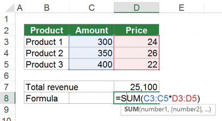
So how to create a simple array formula in Excel? Let’s say you’ve got 3 products, each with amount sold and price as shown in the screenshot on the right-hand side. You want to know the total revenue.

The formula in cell D7 is

{=SUM(C3:C5*D3:D5)}

The curly brackets are added when pressing Ctrl + Shift + Enter. The underlying calculation steps are as follow:

=C3*D3+C4*D4+C5*D5
=300*24+350*26+400*22
=7200+9100+8800
=25100

This is probably an easy example for a single-cell-array formula. Of course, the result can also be achieved with the SUMPRODUCT formula or an additional helper column.

Follow up the calculation steps of array formulas

One recommendation: Because array formulas are often difficult to understand it’s worth noting that the formula auditing tools work for them as well. So you can follow up the calculation steps of an array formula with the formula auditing tools in Excel quite well. In order to achieve this, click on “Evaluate Formula” on the “Formula” ribbon. Now you can see each calculation step.

Delete array formula

When deleting array formulas, you have to differentiate between single-cell- and multi-cell-array formulas.

Deleting single-cell-array formulas is quite simple: Just select the cell containing the array formulas and press the delete key on the keyboard. Alternatively select the cell to delete, click on “Clear” on the Home ribbon and then on “Clear Contents” or “Clear All”.

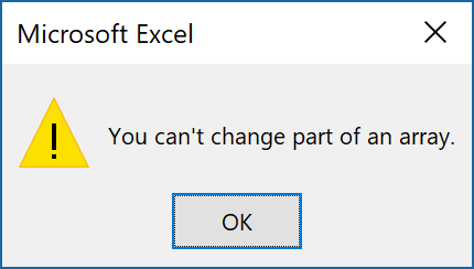
If you want to delete multi-cell-array formulas, you have to work a little bit harder. Instead of just selecting one cell, you have to select all cells belonging to the current array of cells. If you don’t catch all related cells at the same time, you’ll receive the “You can’t change part of an array” error message.

So how to select the whole array (that means all cells belonging to the current multi-cell-array)?

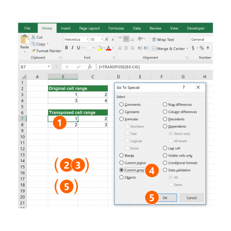
1. Select one cell of your multi-cell-array formula cells.
2. Press Ctrl + G on the keyboard for opening the Go To-window. Alternatively click on “Find & Select” on the right-hand side of the “Home” ribbon and click on “Go To Special”. If you choose this alternative way you can skip the following step three below.
3. Press Alt + S on the keyboard or click on “Special…”
4. Select “Current array”.
5. Click on OK.
6. Press the Delete key on the keyboard or alternatively click on “Clear” on the Home ribbon and then on “Clear Contents” or “Clear All”.

Change the size of an array formula

In practice you have to change the size of an array formula comparatively often. Unfortunately, that is not as simple as it sounds. Single cell array formulas are usually not a problem because you can handle them like normal formula cells. So once again, it’s the multi-cell array formulas that are challenging.

The first approach (and often the fastest way to change the size of multi-cell array formulas) is to delete the complete formula and set it up again from the beginning. Especially in cases with complex array formulas this method might be troublesome. But in such case also the following second approach for resizing array formulas causes similar troubles.

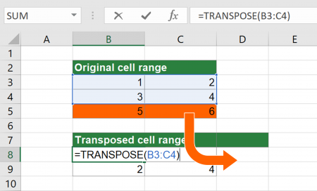
The second approach is use the existing multi-cell array formula, change the cell references within the formula and apply it to the complete cell range. To demonstrate this, please take a look at the following example as shown in the screenshot on the right-hand side.

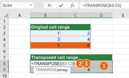
In this example you already have a simple TRANSPOSE formula. It exchanges rows and columns of the cells B3 to C4. The task is to extend it to some new data given in cells B5 and C5 (the highlighted cells).

1.  Start by selecting the new, extended cell range of your TRANSPOSE formula. In this example it’s cells B8 to D9. Please keep in mind that the TRANSPOSE formula exchanges the rows and columns so that if you add one row in the original data you have to add one column for the TRANSPOSE formula.
2. Press F2 on the keyboard for editing the existing formula. Change the cell reference within the array formula manually. In this case replace B3:C4 by B3:C5.
3. Press Ctrl + Shift + Enter on the keyboard.

Please note the following rules for resizing multi-cell array formulas in Excel.

• You can’t shrink multi-cell array formulas in Excel. You can only enlarge them. If you want to make a multi-cell array formula smaller, you have to delete it and set it up from the beginning.
• Moving multi-cell array formulas per drag-and-drop or cutting and pasting them (Ctrl + X and Ctrl + V on the keyboard) is possible, but only the complete cell array at the same time. Moving single cells of multi-cell array formulas is not possible.

---

Do you want to boost your productivity in Excel?

Get the Professor Excel ribbon!

Learn more

Download Free Trial

Add more than 120 great features to Excel!

---

Array constants

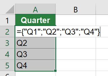
Like non-array formulas (“normal formulas”) you can work with numbers or other values in array formulas, so-called array constants. Array constants are a set of static values that don’t change. They can be used as arguments within array formulas. An example is shown in Figure 86. The constants are embraced by curly brackets and each value is separated by a semi-colon.

You have to manually insert the curly brackets around the array constants. Additionally, you have to press Ctrl + Shift + Enter after editing the formula so that a second pair of curly brackets is added around the whole formula.

We’ve said before that each value should be separated by a semi-colon. A semi-colon in terms of array constants means that all values are in one column. If you instead separate the values with commas, the values are in one row. Now you can combine commas and semi-colons. That way you create two dimensional array constants, similar to an Excel table with rows and columns.

Example: The following formula…

={“Q1 2017″,”Q2 2017″,”Q3 2017″,”Q4 2017″;”Q1 2018″,”Q2 2018″,”Q3 2018″,”Q4 2018”}

…translates into this table:

As you can see the first four value from “Q1 2017” to “Q4 2017” are separated by commas. These values represent the first row. Starting from the semi-colon the second row starts.

Let’s take it to the next level now. So now you know how to handle array constants. Next you can assign a name to the array constant. That way you don’t have to type it again in your array formula but instead only use the array constant by inserting the name into your formula.

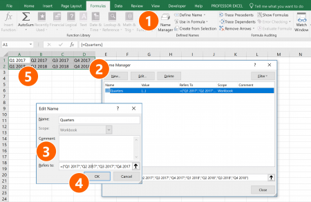
Recommendation: Type your array constant one time directly into an Excel cell and test it. If it works, copy it. Now continue with the following steps (the number relate to the image on the right-hand side).

1. Click on “Name Manager” in the center of the “Formulas” ribbon.
2. Next, click on “New” in order to set up a new name.
3. Type a name in the field “Name:” and paste the previously copied array constant into the field “Refers to:”.
4. Confirm with “OK” and click on “Close”.
5. Now you can use the given name in your Excel formula.

Summary of array formulas

In this article you learned the basics of array formulas. Especially relevant for some special lookups, for example VLOOKUP to the left or VLOOKUPS with several criteria rely on these formulas. Some of these special lookups don’t have a non-array alternative. In such case you have to use array formulas. Furthermore – although probably nowadays not that relevant any longer – you could reduce the file size of Excel workbooks because you can conduct several calculation steps within one formula.

That said it’s time for some disadvantages and words of caution about them.

• Array formulas are comparatively slow in terms of calculation performance. In many cases, you won’t notice the difference but if you use array formulas in great scale it can significantly slow down your workbook’s performance.
• Especially inexperienced Excel users often can’t handle array formulas. Therefore please keep your workbooks audience in mind when you create Excel files.
• Another disadvantage of these formulas is that they are difficult to edit, for example to change the cell arrays.

Download

Please feel free to download the examples from this article in one Excel workbook. Just click here to start the download.