
The SUMPRODUCT formula in Excel is quite powerful. The disadvantage: SUMPRODUCT is often not self-explanatory. Before Excel version 2007 it was used as the SUMIFS formula. Fortunately, with Excel 2007 the SUMIFS formula replaced SUMPRODUCT in many cases. But there are still some cases, in which you have to use SUMPRODUCT. Here is everything you should know about the formula in Excel.
Introduction
The SUMPRODUCT formula sums up all values after multiplying cell ranges with each other.
You might wonder, why this is important in terms of lookups? There are two reasons:
- Before SUMIFS was introduced with Excel version 2007 you could achieve a multi-conditional sum using the SUMPRODUCT formula. Since the introduction of Excel 2007 it’s already more than 10 years so that this usage is a bit outdated. Nonetheless, in this chapter you explore a short example.
- Nowadays you still need the SUMPRODUCT formula for advanced lookups. The best example is the case-sensitive lookup (please refer to this article for more information), which is not supported by the SUMIFS formula.
SUMPRODUCT has one special characteristic. It is not an array formula by definition because it doesn’t require you to press Ctrl + Shift + Enter after typing. However, it deals with arrays so that the usage is quite similar to array formulas.
How does the SUMPRODUCT formula work?

The structure of the SUMPRODUCT formula is quite simple. You just provide at least one and at most 255 ranges of cells as shown in the image on the right-hand side.
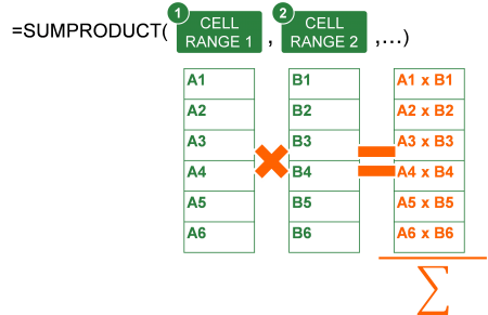
The image on the right-hand side illustrates how the formula works. Say, you have the two ranges A1 to A6 and B1 to B6. SUMPRODUCT multiplies cell A1 with B1, A2 with B2 and so on. Afterwards, it sums up all single result.
Example 1 for the SUMPRODUCT formula
As a first example, you explore the basic usage of the SUMPRODUCT formula: Multiplying to cell ranges and summing up the result.
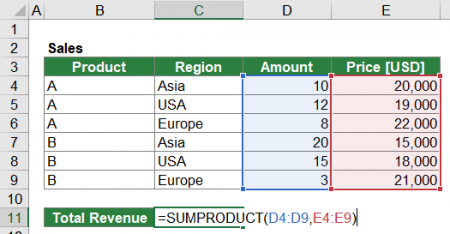
Say, you have sales data as shown in the screenshot on the right-hand side. Besides the product and region, you also have the amount per product and region as well as the price for each combination of product and region. You want to calculate the total revenue.
That means, you have to multiply the amount with the price for each combination of product and region, in this case for each row. You could achieve this with an additional helper column. Alternatively, you could just use the SUMPRODUCT formula.
The SUMPRODUCT formula for this example is shown in cell C11 of the screenshot on the right-hand side. You only have to put both cell ranges (amount and price) into the SUMPRODUCT formula. The resulting formula is
=SUMPRODUCT(D4:D9,E4:E9) .
Example 2 for the SUMPRODUCT formula
Besides the basic usage as shown in the previous example, you can use the SUMPRODUCT formula for lookups. The basic idea is that you multiply ranges by 1 if a condition is met and by 0 if not.
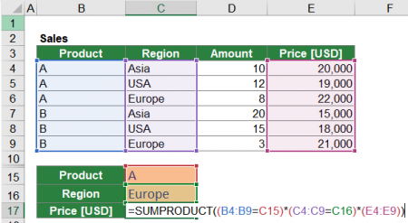
Please take a look at the image on the right-hand side. You have a simple table listing products and regions in columns B and C as well as the price listed in column E. You want to return the price from column E by selecting a product and region.
The approach is quite simple.
- You combine all the criteria with the *-sign.
- Embrace each criteria by brackets.
- Criteria have this form: (criteria_range=criteria).
- The return range (which contains the value to return) is added without any = (equal) sign.
Applying this on the example above leads to the following formula:
=SUMPRODUCT((B4:B9=C15)(C4:C9=C16)(E4:E9))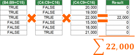
Here is what happens in the background: Through the multiplication of each argument, TRUE arguments are converted to the number 1 and FALSE arguments to 0. Only if all arguments return TRUE (which means 1), the product is not 0. In the example above, that’s only the case for the third row so that the result is 22,000.
Please note: The arguments of the SUMPRODUCT formula can also be entered slightly different. Instead of using the *-sing, you can separate the arguments with a comma. In this case you have to make sure that the resulting TRUE and FALSE arguments are converted to number by either multiplying them by 1 or using the double minus sign (“–“). The formula could look like this:
=SUMPRODUCT(--(B4:B9=D15),--(C4:C9=D16),E4:E9)Example 3 for the SUMPRODUCT formula
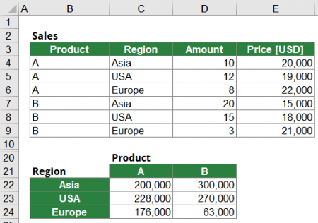
In a third example for the SUMPRODUCT formula you want to combine the previous two examples. The goal is to return the sum of products if two criteria are fulfilled like shown on the image on the right-hand side.
You want to multiply the amount of each product and region by the price. The result is the revenue for each product and region. Please follow the same rules as before:
- You combine all the criteria with the *-sign.
- Embrace each criteria by brackets.
- Criteria have this form: (criteria_range=criteria).
- The return ranges (which contain the value to multiply and return) is added without any = (equal) sign.
Applying these rules on the example above results in the following formula (cell C22):
=SUMPRODUCT(($B$4:$B$9=C$21)($C$4:$C$9=$B22)($D$4:$D$9)*($E$4:$E$9))The calculation steps for the fomula in cell C22 are shown in the picture on the right-hand side.
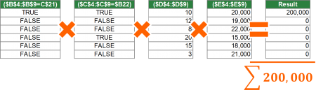
Also in this case, you can slightly transform the formula and divide each argument by comma.
=SUMPRODUCT($D$4:$D$9,$E$4:$E$9,–($C$4:$C$9=$B28),–($B$4:$B$9=C$27))
Download

Please feel free to download all examples above in this Excel workbook. Click here and the download starts.
2nd one did not work its showing value