Case-Sensitive Lookups in Excel: 4 Methods (+XLSX-Download)

By definition, the VLOOKUP formula is not case-sensitive. Case-sensitive means, that it matters if you use capital letters or small letters. For instance, a VLOOKUP search for “AAA” will return the same value as for “aaa” or “Aaa”. But in some cases, you want to differentiate between capital and small letters. So how do you proceed? In this article, you learn how to make VLOOKUP, HLOOKUP, INDEX/MATCH and SUMIFS case-sensitive.

Example for all methods

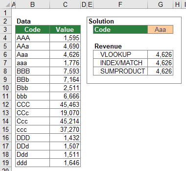
All following methods will be introduced with the example as shown in the image on the right-hand side. The cell range B4 to B19 contains codes (e.g. “AAA”, “AAa”, and so on) and the cell range C4 to C19 contains numeric values. In cell G3 you can insert a code (e.g. “Aaa”). The goal is to return the numeric value from the cells C4 to C19, depending on the code given in cell G3. For example if the code in G3 is “Aaa” you want to return the value from cell C6, which is 4,626.

Method 1a: Case-sensitive VLOOKUP

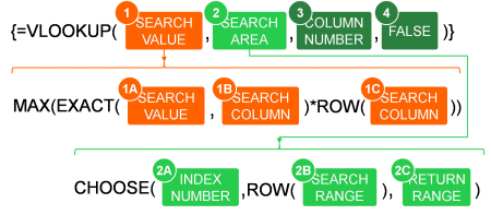
The first method is based on the VLOOKUP formula. Unfortunately, the approach is a little bit complex and only works through a workaround. The structure of the case-sensitive VLOOKUP is shown in the image on the right-hand side.

The underlying idea is not to conduct a VLOOKUP with the actual search value, but rather with the row number, in which the search value can be found.

1. SEARCH VALUE: This part of the formula identifies the row number. It comprises several formulas. The part EXACT()*ROW() returns an array of row numbers which match the search value. From this array, the embracing MAX formula just identifies the largest row number.
   1. SEARCH VALUE (within the EXACT formula): This is the actual value you look for.
   2. SEARCH COLUMN: The column you search in. It’s typically the leftmost column of your VLOOKUP formula.
   3. SEARCH COLUMN: Again, the same cell reference like the previous argument.
2. The SEARCH AREA creates an array (like a table with two columns) which contains the row numbers in the first column and the return values in the second column.
   1. INDEX NUMBER: In case of such lookup, the INDEX NUMBER is always {1,2}.
   2. SEARCH COLUMN: The range of cells in you search in as before in 1B and 1C.
   3. RETURN COLUMN: The column that contains the value you want to get returned.
3. The COLUMN NUMBER is in case of this exact VLOOKUP always 2. The reason is that from the virtual table created with the CHOOSE formula you need to return the value from the second column.
4. As usual, the last argument of the VLOOKUP formula is FALSE because you want search for the exact value.

Please note: As for all array formulas please press Ctrl + Shift + Enter on the keyboard after typing the formula.

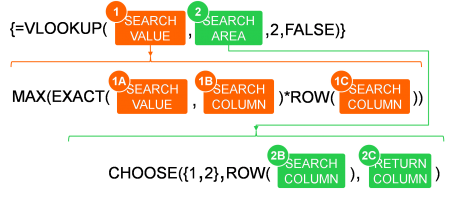
If you insert the fixed arguments into this formula, you get the simplified structure of the VLOOKUP formula in the image on the right-hand side.

For our example, the case-sensitive VLOOKUP has the following parameters:

• SEARCH VALUE: The search value is given in cell G3.
• SEARCH COLUMN: You search in the cell range B4 to B19.
• RETURN COLUMN: You want to get the value from cell range C4 to C19 returned.

Putting these parameters into the formula structure of Figure 93, you get the following formula.

{=VLOOKUP(MAX(EXACT(G3,B4:B19)*(ROW(B4:B19))),CHOOSE({1,2},ROW(B4:B19),C4:C19),2,0)}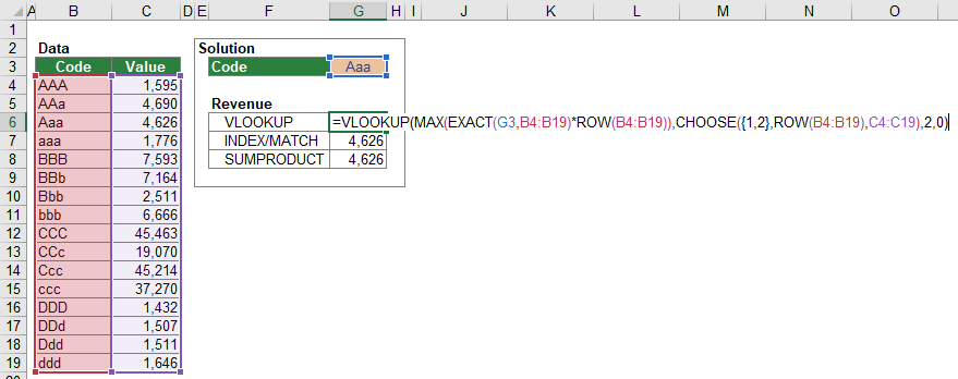

Method 1b: Case-sensitive HLOOKUP

A case-sensitive HLOOKUP works very similar to the VLOOKUP. The only difference is that you have to insert 3 TRANSPOSE formulas around and inside the CHOOSE formula. The reason is that CHOOSE can only handle vertical cell ranges in this case.

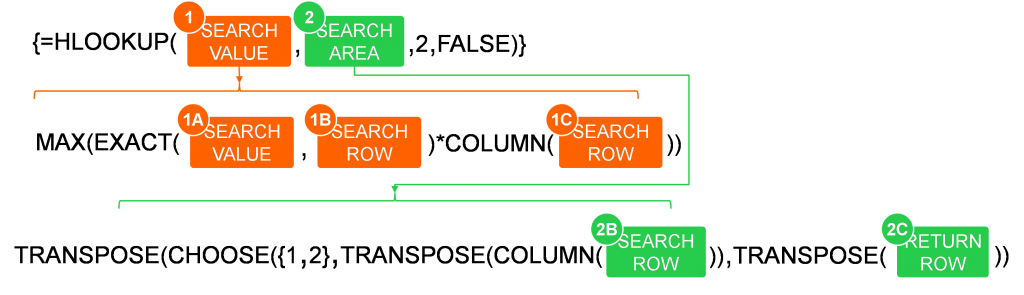
The structure of the case-sensitive HLOOKUP formula is shown in the image above. As you can see, the formula is getting quite long. This might be a good example for a possible solution in Excel, but not necessarily the best one. The following method number 2 is usually a better option for a case-sensitive, horizontal lookup.

The arguments of the HLOOKUP formula are pretty much the same as in method 1a, the VLOOKUP formula. Applying this to a very similar example leads to the following formula.

{=HLOOKUP(MAX(EXACT(D7,C3:R3)*COLUMN(C3:R3)),TRANSPOSE(CHOOSE({1,2},TRANSPOSE(COLUMN(C3:R3)),TRANSPOSE(C4:R4))),2,FALSE)}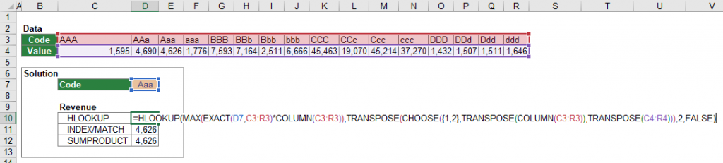

Method 2: Case-sensitive INDEX/MATCH

The case-sensitive INDEX/MATCH formula is compared to the case-sensitive VLOOKUP formula quite simple. The INDEX/MATCH formula is shorter and in many cases the better option.

The structure of the case-sensitive INDEX/MATCH formula combination is shown in the image on the right-hand side, the following number relate to the image.

1. RETURN RANGE: The range of cells containing the return value. This can be a vertical range (in case you use the INDEX/MATCH formula vertically) or a horizontal range of cells.
2. The LOOKUP VALUE is a little bit different than usual. Because the next argument (number 3) checks for each cell if it equals exactly (that means case-sensitive) the search value and returns an array of cells containing TRUE or FALSE for each cell, your LOOKUP VALUE is always TRUE for case-sensitive lookups.
3. The LOOKUP RANGE is usually the range of cells you search in for your lookup value. For a case-sensitive INDEX/MATCH formula combination, you create an array of cells (a virtual table) which contains only TRUE or FALSE. TRUE, if the SEARCH VALUE matches exactly the value of a cell in the SEARCH RANGE and FALSE, if not.
   1. The SEARCH VALUE is the value or cell reference you are looking for.
   2. The SEARCH RANGE contains the cells you are looking in.
4. Because you want to get an exact match, the last part of the MATCH formula is 0.

Please note (again): As for all array formulas please press Ctrl + Shift + Enter on the keyboard after typing the formula.

The structure shown in Figure 94 can be simplified. After inserting the fixed arguments, the INDEX/MATCH formula looks like in the image on the right-hand side.

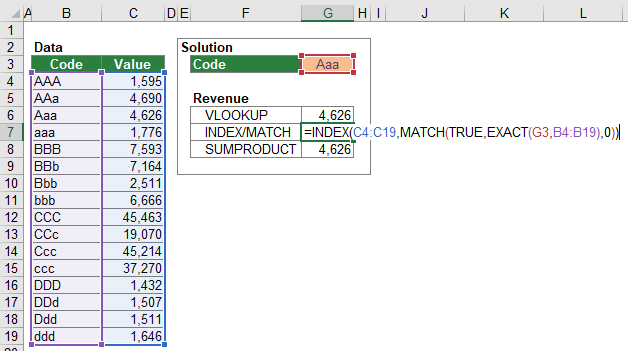
Applying this structure on our example, you have the following parameters.

• RETURN RANGE: You want to return the value from the cell range C4 to C19.
• SEARCH VALUE: The search value is given in cell G3.
• SEARCH RANGE: You search in cell range B4 to B19.

If you now put these parameters into the structure, you get the following formula.

{=INDEX(C4:C11,MATCH(TRUE,EXACT(G3,B4:B11),0))}

Method 3: Case-sensitive SUMPRODUCT instead of SUMIFS

The SUMIFS formula doesn’t support an exact lookup. That’s why you could use an alternative formula instead: SUMPRODUCT. Although no “real” array formula (with curly brackets), the SUMPRODUCT formula works like an array formula because it deals with arrays.

The structure of the case-sensitive SUMPRODUCT formula is shown in the image above. The SUMPRODUCT formula multiplies all arguments with each other and sums up the results. If a criterion is not fulfilled, the argument is 0 so the result of the multiplication is 0.

• SEARCH VALUE: The value or cell reference you look for.
• SEARCH RANGE: The range of cells you look in.
• RETURN RANGE: The range of cells from which you want to get a value returned.

Because this formula is not an array formula, you don’t have to press Ctrl + Shift + Enter when finished typing.

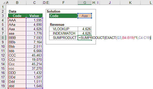
For the example of this chapter, you will get this SUMPRODUCT formula (also shown in the image on the right-hand side.

=SUMPRODUCT(EXACT(G3,B4:B19)*1,C4:C19)

Please note: The SUMPRODUCT approach only works with numeric return values (including dates). If your return value is a text or string, SUMPRODUCT doesn’t work.

Download

Please feel free to download an Excel workbook with all the examples from this article. Just click on this link and the download starts immediately.