Working with other people on the same Excel file can be challenging. Especially when you prepare an Excel workbook and another person has to fill in some data. In such case, you probably want to make sure that only your intended values are possible to enter. In this article we learn how to restrict cells to certain values with the data validation function, including adding drop-down lists. Furthermore we’ll take a look at the example of a cell in which the user has to fill in a complete form.
In a hurry? Click here to scroll down to the drop-down list guidance.
Basics of the data validation function in Excel
Excel provides the “Data Validation” function. With Data Validation, you can define, what values or what type of values are allowed for each cell (e.g. date, whole numbers).
Steps for adding restrictions to a cell
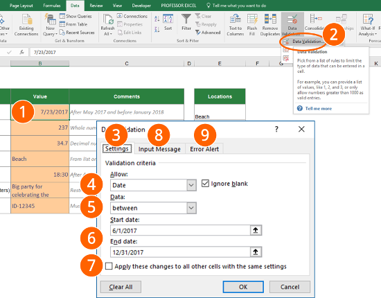
In order to restrict cells to certain numbers or values, please follow these steps (the numbers are corresponding to the picture above):
- Select the cell(s) you want to limit.
- Click on “Data Validation” in the middle of the Data ribbon. Alternatively, press Alt –> A –> V –> V on the keyboard.
- Within the settings tab you can define the allowed values.
- Let’s say, you want people to enter their date of birth. So there are two limitations: It must be a date and it can’t be any day later than today. Select “Date” on the dropdown list.
- As we want to limit the maximum value, we have to select “less than” at “Data:”.
- The end date can either be a fixed date or a formula. In our case we go with the TODAY formula.
- If you want to give a hint about what data is allowed to fill in, you can set an input message (see below for more information)
- If someone enters a value which is not allowed (for example a date in the future or text), you can define an error message, as well as the message type.
Update all cells with the same settings
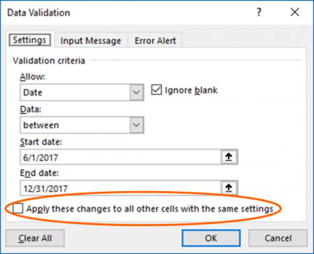
Excel offers the option that you update all cells with the same settings. That’s very helpful – you don’t have to find and select all cells you want to change. Just set the tickmark like on the screenshot on the right side.
Input Message: Provide some help to the user
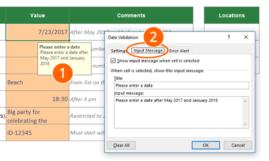
Your co-worker or client who has to fill out your form will thank you: Provide some help. When you select a cell, a small yellow field will appear with your help text (number 1 on the picture).
In order to set up an input message follow these steps:
- Open the data validation window again by clicking on “Data Validation” in the center of the Data ribbon.
- Go to the “Input Message” tab (number 2).
- Make sure the tick is set for “Show input message when cell is selected”.
- Type your text below for a title and the actual input message.
- Confirm with OK.
Error message for wrong inputs
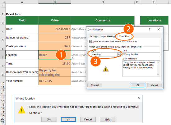
You can also give your own error message, if someone enters a wrong value. You can even select the style:
- Select the cell you want to provide the error message for (number 1 on the screenshot).
- Open the data validation window again by clicking on “Data Validation” in the center of the Data ribbon.
- Go to the “Error Alert” tab (number 2).
- Select your style (number 3). You got 3 options:
- Stop:

- Warning:

- Information:

Important: If you choose warning, the user can choose to still use his “wrong” value. For stop or information, the user can’t.
- Stop:
- Type a message title as well as the error message.
- Confirm with OK.
Example: Prepare a form
Let’s take a look at an example with many different data validation rules.
The task
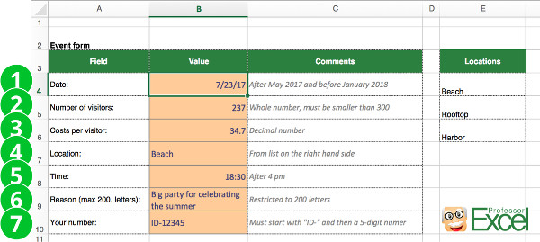
You want to restrict all the input cells (the beige cells). The user has to be restricted:
- The date of the event should be between May 2017 and December 2018.
- The number of visitors has to be a whole number and should be smaller than 300.
- The costs per visitor should be a decimal number less than 100.
- The location should be selected from the list on the right hand side.
- The time should be after 4 pm (16:00).
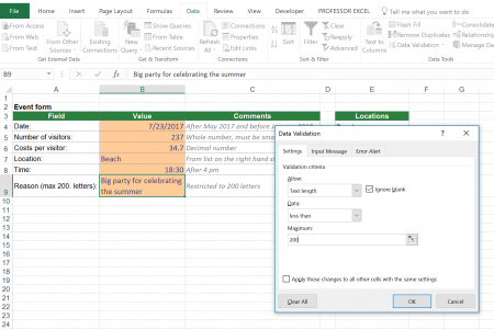
- The maximum length of the text (in this case the reason) reason should not restricted to 200 characters.
- Your ID number. This one is special as it should start with “ID-” and being followed by a 5-digit number. Therefore you have to choose the option “formula“.
The solution (including drop-down lists)
Please feel free to download the example workbook here.
Only allow a certain date or date range
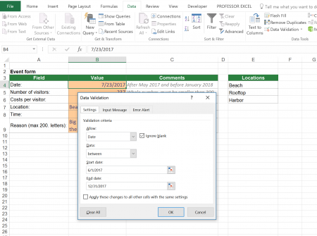
Select “Date” under “Allow:”. Under “Data” select “between” if you want to set a start and end date.
Click on the image to see it large or download the example workbook here.
Only allow whole numbers
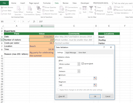
If you want to allow whole numbers only, select “Whole number” under “Allow:”. Furthermore, you can set a minimum and maximum if you choose “between” under “Data:”.
Click on the image to see it large or download the example workbook here.
Only allow a number range between decimal numbers
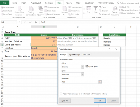
3) Very similar to whole number is the allow option “Decimal”. In this example there is only a maximum defined.
Click on the image to see it large or download the example workbook here.
Only allow items from a drop-down list
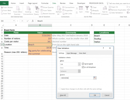
4) This option is most popular: The user can select an item from a drop-down list. Therefore, you have to allow “List” and link to the list in Excel. Alternatively, you can write the possible values directly into the “Source” field, separated by commas.
Confirm with “OK” and your cell now has a drop-down lists.
Click on the image to see it large or download the example workbook here.
Only allow a certain time
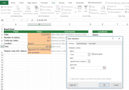
5) If you want to restrict a time, you can do so by allowing “Time”. Set the Start time in the format “00:00”.
Click on the image to see it large or download the example workbook here.
Only allow a maximum number of characters
6) Some people tend to write a lot. You can restrict that by allowing a maximum number of letters.
Click on the image to see it large or download the example workbook here.
Do you want to boost your productivity in Excel?
Get the Professor Excel ribbon!

Add more than 120 great features to Excel!
Only allow anything you want with a formula
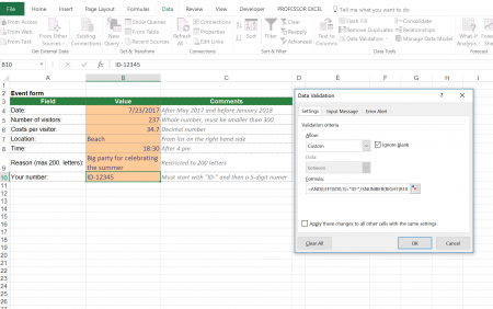
7) The most complicated option: Use a formula to restrict input values. In this case the input value must start with “ID-” and must be followed by a 5-digit number. The complete formula is: =AND(LEFT(B10,3)=”ID-“,ISNUMBER(RIGHT(B10,5)*1))
Click on the image to see it large or download the example workbook here.
Final comments
- Please note that the data validation rules aren’t copied with the format painter. Instead, you can copy the cell, paste it with “Paste Special” and select “Validation” on the paste special window.
- Data validation can be quite troublesome when copying sheets from one workbook to another. When you link the condition to another place in the original workbook, you can’t use the “Break links” function (well, you can but it doesn’t work). Please refer to this article in such case.


