Precedents and Dependents: Easily Trace Related Cells in Excel

Let’s assume the following situation: You receive an Excel file from your colleague and have to understand it as quickly as possible. How do you start? In this article we’ll learn how to trace depending and preceding cells in Excel. The functions in Excel are called “Trace Dependents” and “Trace Precedents”.

Functions “Trace Dependents” and “Trace Precedents”

Basic usage

Here is how the basic functions of tracing depending and preceding cells.

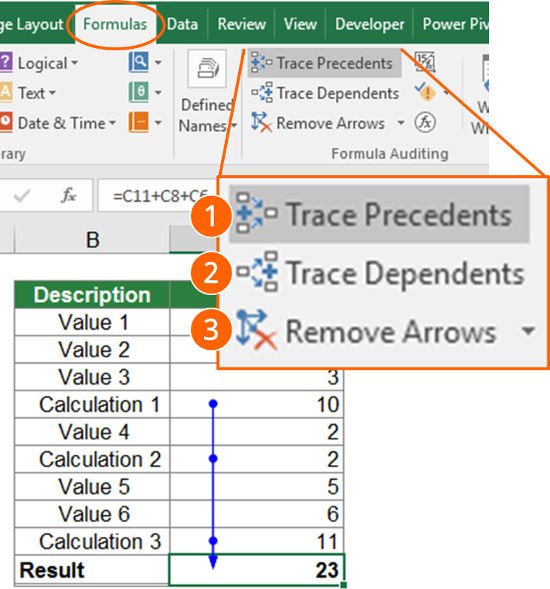
• Before you start, select one cell. In the example on the right-hand side, it’s the result in cell C12.
• Then go to the “Formulas” ribbon.
• Within the “Formula Auditing” group, you have the following three choices.

1. By clicking on “Trace Precedents”, blue arrows show the direct input cells. By clicking it the button again, the input cells of these input cells will also be shown and so on.
2. The same way you can see the cells, which use the current cell as an input value. Just click on “Trace Dependents” for displaying the arrow in the opposite direction.
3. By clicking on “Remove Arrows”, all arrows will be hidden.

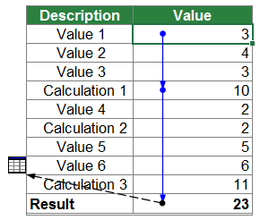
Please note, that a black dotted arrow with some table symbol indicates, that some input cells are located on another worksheet. Double-click on the black dotted arrow and then double-click on one of the list entries to see the corresponding input cell.

Show all dependents and precedents for multiple cells simultaneously

Unfortunately, you can’t check the relations of multiple cells at the same time. Even if you select a cell range and click on on either “Trace Precedents” or “Trace Dependents”, only the arrows for one cell will be displayed. However, the following short VBA macros help you to highlight all relations of a selected cell range.

Sub showAllPrecedents() 
    Dim cell As Range
    For Each cell In Selection
        cell.ShowPrecedents 
    Next cell 
End Sub

Sub showAllDependents()
    Dim cell As Range
    For Each cell In Selection
        cell.ShowDependents
    Next cell
End Sub

Follow these steps to use the code above:

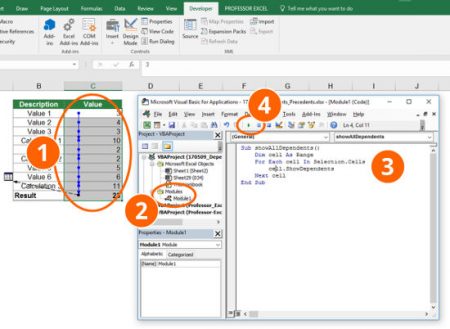
1. Select a range of cells. Please keep in mind that there should be formulas within the selected cells. Otherwise you won’t see any arrows.
2. Open the VBA editor by pressing Alt + F11 on the keyboard. Insert a new module.Please refer to this article for a description of how to insert a module.
3. Copy and paste the code above into a VBA module. Place the cursor into one of the “SUBS”:
   1. Move the cursor to showAllPrecedents if you want to display the arrows of all preceding cells.
   2. If you on the other hand want to see all dependents, place the cursor into the SUB showAllDependents.
4. Click on start on the top of the editor window.

---

Do you want to boost your productivity in Excel?

Get the Professor Excel ribbon!

Learn more

Download Free Trial

Add more than 120 great features to Excel!

---

Clear all arrows from all workbooks at the same time

Please use this short VBA macro to clear all blue arrows from all worksheets simultaneously.

Sub clearAllArrowsInCurrentWorkbook()
    Dim ws As Worksheet
    For Each ws In Worksheets
        ws.ClearArrows
    Next ws
End Sub

Just copy and paste this code into a new VBA module, place the cursor into the code and press the play button on top of the VBA editor window. If you need assistance with VBA macros, please refer to this article.

For experts: Use Professor Excel Tools

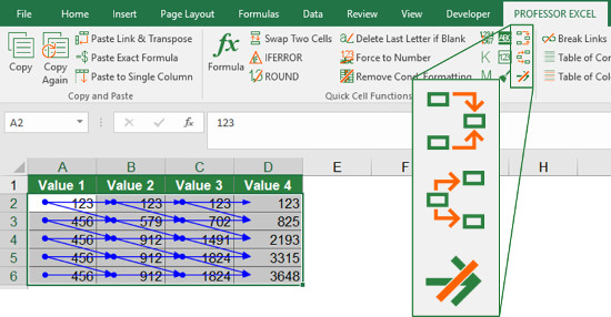
You want to simplify this process? Use Professor Excel Tools. The Excel add-in helps you to

• show all precedents of the selected cells,
• show all dependents of the selected cells and
• hide all arrows from all worksheets.

Just select the cells you want to highlight the precedents and dependents of and press the button of Professor Excel Tools.

Try Professor Excel Tools for free now. Click here to learn more!

---

This function is included in our Excel Add-In ‘Professor Excel Tools’

Learn more

Download Free Trial

(No sign-up, download starts directly)

More than 35,000 users can’t be wrong.

---

How to check, if a cell is used in another formula

Here is another use of this functions to trace precedents. Sometimes you want to delete a cell (or a certain worksheet), but you are not sure if you still need that cell. You have to differentiate various types of dependent cells.

Types of dependents

1. The cell is directly linked or referred to. For example, cell A1 might be used within a formula in cell B1 in such way =A1+A2 or within a formula, e.g., =SUM(A1:A2).
2. The cell is indirectly linked to, e.g. with the INDIRECT or OFFSET formula. Also VLOOKUP and HLOOKUP might use your cell as a return value.
3. The cell is used in a VBA macro.
4. Cell is used in a defined name.
5. Cell is part of the source of a chart.
6. Cell is part of the source of a PivotTable.
7. The cell is referred to by another workbook.
8. The cell is used in a conditional formatting rule.

Unfortunately, only the first of the types above can be checked with the “Trace Dependents” formula.

Check if cell is direct input to another cell

Concerning item 1 above: You could use the “Trace Dependents” function to check, if your selected cell serves as an input for another cell. Just select the cell and click on “Trace Dependents”. If the error message “The Trace Dependents command found no formulas that refer to the active cell” (6) appears after clicking on “Trace Dependents”, you could most probably delete that cell.

Strategies to check if cell is referred to by an INDIRECT or OFFSET formula

Concerning item 2 above: Unfortunately, there is no universal way of checking, if a cell is still in use by another INDIRECT or OFFSET formula. But you could use some rather rough approaches.

1. Check if your workbook has are any INDIRECT or OFFSET formulas. You could do this by searching for “INDIRECT” on all worksheets. If there are no INDIRECT formulas in your workbook, you can stop here. Do the same for OFFSET.
2. If there are just a small amount of INDIRECT formulas in your Excel workbook, change the value within the cell in question and check if any of your INDIRECT values change. This method is unfortunately not 100% safe because the cells with the INDIRECT formula might not change the value (e.g. through the IF- of IFERROR formulas).