FIELDVALUE Formula in Excel: Insert Data of Companies and Countries (+Download)

Excel has – in it’s newest version – a quite useful new formula type. It’s called “linked data” and offers the functionality to automatically insert data from the internet to your table. This can be done with the FIELDVALUE formula and works in a first test quite well. Unfortunately, the available data types and options are limited so far. But let’s see how it works first.

The FIELDVALUE formula

The FIELDVALUE formula retrieves data from the internet (from so-called linked records) and adds them to your table. So far, the FIELDVALUE formula works for two types of data:

1. Data of companies and
2. data about geographic regions such as countries, cities or states.

Requirements and preparation

In order to use the FIELDVALUE formula, you have to prepare your data in a certain way. Because it only works with company names or geographic region names, you have to select a cell containing a company name or country name and define it as such. The following steps are shown for region names but they work the same way for companies.

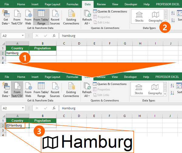
1. Type a country or region name into an Excel cell, for example “Hamburg” (a city in Germany). It doesn’t work if the cell is empty.
2. Go to the “Data” ribbon and click on “Geography” in the “Data Types” section. (Please note once again that this function is by now only available for the newest version of Excel – in Mai 2018 only in the insider channel.)
3. If the geographic region is found, a small map symbol is shown in the cell.

That’s it in terms of the preparations. In the next paragraph you learn how to pull data of a geographic region into an Excel cell.

Structure of the FIELDVALUE formula

In the previous paragraph you’ve learned how to prepare your Excel cell in order to retrieve data about a geographic region (or company). Now we continue by inserting the actual data. This is done using the FIELDVALUE formula.

The structure of the FIELDVALUE formula is shown on the right-hand side. It has only two arguments. The value and the field name.

1. The value refers to your geographic region or company name. Just link to the cell which you’ve before defined as “Geography” or “Company”. Just typing “Hamburg” (or any other region or company name) directly into the formula doesn’t work.
2. Select the data type you want to pull from the internet and insert into your Excel cell. For example, type “Population” in order to retrieve the number of inhabitants of Hamburg (by the way, it’s 1,787,408 😉 ).

Refer to data types without the FIELDVALUE formula

Excel also provides another method to refer to data types. This method avoids the FIELDVALUE formula, but it still has the same two arguments like the FIELDVALUE formula. The structure is shown in the image on the right-hand side.

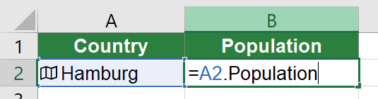
As for using the FIELDVALUE formula you have to prepare one cell by defining it as data type “Stock” or “Geography”. Now you can just refer to this cell (e.g. =A2) and adding the field name (e.g. population) with a “.”. Say you want to know the population of the city “Hamburg” and the city name “Hamburg” is given in cell A2. You simply type =A2.Population .

Please note: If your FIELD_NAME contains ” ” space characters, you have to put [ ] around the field name. Example: =A2.[Population: Income share third 20%]

Even easier: Let Excel do the work for you

You actually don’t even have to type the FIELDVALUE formula or the simplified version as shown above yourself. Excel can do that for you. One condition: Your table has to be formatted as an Excel table.

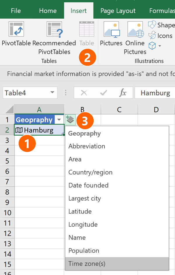
1. Convert your table into an Excel data table. In order to achieve this, select any cell within your table, click on “Insert” and then on “Table”. Follow the steps on the screen. (Please don’t be confused: In the screenshot on the right-hand side, the “Table” button is greyed-out because the data is already formatted as an Excel table.)
2. Make sure that the company or geography identifier (that means, the cell having your company or region name) is set to the corresponding data type “Stock” or “Geography”. If it is, a small symbol is shown indicating that the data type is either “Stock” or “Geography”.
3. Now Excel offers a small button with a plus sign and “layer”. If you click on it you can see all the data available. Just click on any entry and Excel adds a new column contain the desired data.

Examples

Let’s take a look at two examples. In the first example we are going to retrieve data for countries. The second example is about pulling take of companies.

Pull data about countries

The goal: Get some basic data about countries, e.g. the population, area size, year established or the name and position of their leaders.

1. Prepare a table containing rows and columns. In this example, we’ll have one column for each countries and the row contain the different data types.
   1. Cell A1 should say “Country”.
   2. Cell B1 can already contain the first country name, e.g. “Denmark”.
2. Convert the country name to a data type “Geography”. In order to achieve this, select cell B1 and click on “Geography” in the center of the “Data” ribbon.
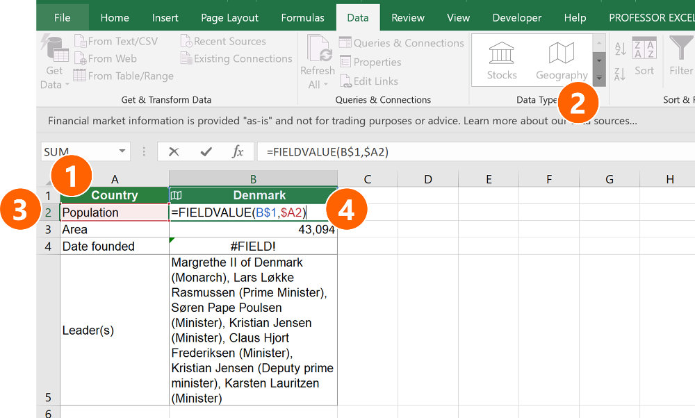
3. In the first row of data (that means row 2 because row 1 contains the column headers) you want to retrieve the population. So cell A2 should say “Population”.
4. Now you can type the actual formula for pulling the required data. In this case (in cell B2) it’s =FIELDVALUE(B$1,$A2) . You don’t have to use the $-signs but if you want to extend this formula later-on, it’s easier to just copy and paste it.

You can now add more columns or rows as shown in the screenshot above.

Pull data about companies

Inserting data about companies into your Excel sheet works almost the same way as for geographic regions. The only difference: You have to set your cell containing the company name to the linked data type “Company”.

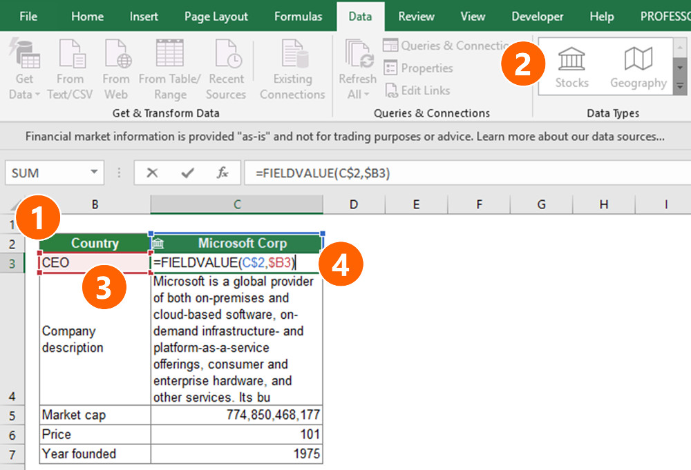
1. Again, prepare the table with rows and columns. Like in the screenshot above select the cell containing the company name (in this case cell C2)
2. Next, set the data type to “Stock” by clicking on “Stocks” in the center of the “Data” ribbon.
3. Let’s start with inserting the name of the CEO. Type “CEO” in cell B3.
4. Now you can insert the actual FIELDVALUE formula into cell C3. In this case it’s =FIELDVALUE(C$2,$B3) .

Errors and limits

#FIELD! error

Coming with the new FIELDVALUE formula, Excel also has a new error type. When typing the formula you might receive the #FIELD! formula. In such case, please check the following things:

• Is your VALUE (the first argument of the FIELDVALUE formula) really a company or region name?
• The FIELDVALUE doesn’t have all data for a company or country. It’s possible that the data for that particular field is simply not available.

PivotTables, Power Pivot and Power Query with linked data types

Microsoft says that PivotTables, Power Pivot, Power Query or even some charts won’t work well with the new data types. However, in a short test, at least PivotTables seemed to work. Maybe you just give it a try…?

English only

As of now, you have to set English to your editing language of Office. Other languages aren’t supported. Microsoft promises to support more languages in the future, though.

Limits

For now, the data itself is very limited.

• Data types are limited. Also the available data is quite limited. Of course, stock quotes might be important for you. But (at least for me when evaluating companies) I need a lot more information: For example the last years revenues, costs, profit margin and so on.
• Data options are limited. The first limit is that you don’t have options for your data. For example, you can only insert the available options of stock quote. You can not define the date and time you’d like to receive the stock quote from.
• Data is missing. It seems as if even major data is missing. For example the year founded of Apple and Amazon. Or the “Official Name” of the USA. But hopefully, Microsoft will improve the integrity of the data over time.
• Available data is incomplete. Our previous limit was that some data is simply missing. But even if data is available, it might be incomplete. For example the business description seems limited to 200 characters.

List of all FIELDVALUE data types

The following data types are currently available.

Geography

Stock

Abbreviation Agricultural land (%) Area Armed forces size Birth rate Calling code Capital Carbon dioxide emissions CPI CPI Change (%) Currency code Date founded Electric power consumption Fertility rate Forested area (%) Fossil fuel energy consumption Gasoline price GDP Gross primary education enrollment (%) Gross tertiary education enrollment (%) Health expenditure as % of GDP Infant mortality Largest city Leader(s) Life expectancy Market cap of listed companies Maternal mortality ratio Minimum wage Name National anthem Official language Official name Out of pocket health expenditure (%) Physicians per thousand Population Population: Income share fourth 20% Population: Income share highest 10% Population: Income share highest 20% Population: Income share lowest 10% Population: Income share lowest 20% Population: Income share second 20% Population: Income share third 20% Population: Labor force participation (%) Subdivisions Tax revenue (%) Time zone(s) Total tax rate Unemployment rate Urban population

Beta CEO Change Change (%) Company description Employees Exchange Exchange abbreviation Headquarters High (52-week high and low values are calculated from close price data.) Industry Instrument type Last trade time Low (52-week high and low values are calculated from close price data.) Market cap Name Open P/E Previous close Price Shares outstanding Ticker symbol Volume Volume average Year founded

Sources

Geography	Stock
Wikipedia Wikitravel CIA (World Factbook)	Morningstar Inc

Download

 Please feel free to download the examples above in one Excel file. Just click on this link and the download starts. Please note: If you get a #VALUE error message it’s possible that your Excel version doesn’t support the new data types yet.