FIND & SEARCH in Excel: How and When to Use These Formulas

The two formulas FIND and SEARCH in Excel are very similar. They search through a cell or some text for a keyword or character. Once found, they return the number of characters, at which the keyword starts. Let’s learn how to use them and explore the differences of the two formulas.

How to use the FIND formula

The formula returns the number of the character, at which your search term starts. If your text can’t be found, it’ll return a “#VALUE” error.

Structure of the FIND formula

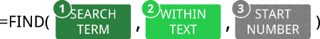
The structure of the FIND formula is quite simple (the numbers are corresponding to the image on the right-hand side):

1. SEARCH TERM: The first part of the formula is the text you look for.
2. WITHIN TEXT: The cell or text you want to search your “SEARCH TERM” in.
3. START NUMBER: This argument is optional. If you don’t want to start searching at the beginning of the text, fill in the number larger than 1, otherwise just type 1 or leave it blank.

If you just want to know, if your text can be found within another cell, you might want to go with the following formula. B2 contains the text or character you search for and B3 is the cell you search in:

=IFERROR(IF(FIND(B2,B3)>0,”Value found”,””),”Value not found”)

Please note the following comments:

• FIND is case-sensitive. That means, it matters if you use small or capital letters.
• You can also search for numbers within another number. For example: =FIND(1,321)This formula returns 3 because the number 1 is the third character of 321.
• You can’t use wildcard criteria (“*” or “?”) with the FIND formula.
• Please refer to this article if you want to know more about the IF formula and to this article for more information about the IFERROR formula.

Examples for the FIND formula

Let’s try some examples.

Example 1: Find the first occurrence

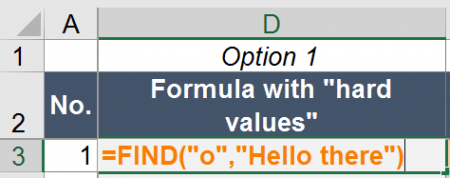
The “default” usage of the FIND formula is to return the number of characters, at which a text first occurs within another text. Let’s say you have the text “Hello there” and want to know, at which position you have an “o”. In such case, you write the following formula (example number 1 in the Excel workbook you can download at the end of this article).

=FIND(“o”,”Hello there”)

The return value is 5.

Example 2: Find the first occurrence after the third character

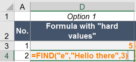
Another example: You want to know the position of “e” after the third character (example number 2 in the example workbook).

=FIND(“e”,”Hello there”,3)

The return value is 9.

Example 3: Find the second occurrence

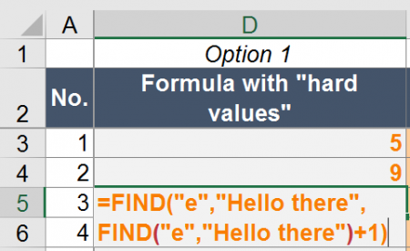
Now you want to know the position of the second occurrence of “e” in “Hello there”.

=FIND(“e”;”Hello there”;FIND(“e”;”Hello there”)+1)

This formula works as follows. The second FIND formula returns the position of the first occurrence of “e” in “Hello there” which is 2. This is used as the START NUMBER (+ 1 because you want to start counting after the first “e”) for the first FIND formula.

Example 4: Find the last occurrence

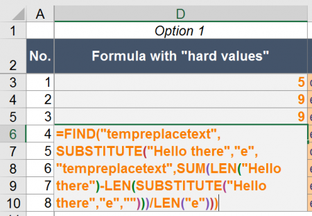
Finding the last occurrence of a string within a text is a little bit more complicated. You use SUBSTITUTE and LEN. The complete formula is like this:

=FIND(“tempreplacetext”;SUBSTITUTE(“Hello there”;”e”;”tempreplacetext”;SUM(LEN(“Hello there”)-LEN(SUBSTITUTE(“Hello there”;”e”;””)))/LEN(“e”)))

In order to understand the formula better, let’s start in the middle with the part SUM(LEN(“Hello there”)-LEN(SUBSTITUTE(“Hello there”;”e”;””)))/LEN(“e”)))

This part of the formula determines the number of “e” in “Hello there”. It replaces “e” in “Hello there” and the difference in the two versions (with and without e – “Hello there” and “Hllo thr”) is the number of “e”s.

The whole part SUBSTITUTE(“Hello there”;”e”;”tempreplacetext”;SUM(LEN(“Hello there”)-LEN(SUBSTITUTE(“Hello there”;”e”;””)))/LEN(“e”))) replaces the last “e” by “tempreplacetext”. Now you just put this into the FIND formula and get the position of “tempreplacetext”.

If you want to use this formula, replace all “e”s by your cell reference for the SEARCH TEXT and all “Hello there” by the cell reference to your WITHIN TEXT.

Replace text enclosed by brackets

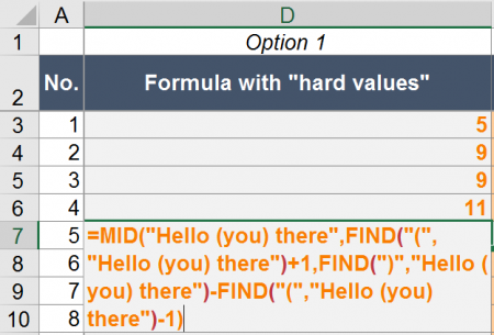
A last example for the FIND formula: You want to know what is written between two brackets. In such case, you can also use the FIND formulas in combination with the MID formula.

=MID(“Hello (you) there”,FIND(“(“,”Hello (you) there”)+1,FIND(“)”,”Hello (you) there”)-FIND(“(“,”Hello (you) there”)-1)

The MID formula returns some part of text from a (longer) text. It has three arguments:

1. The initial, complete text.
2. The starting character for the text you want to get.
3. The length (in number of characters) of text you want to extract.

In our example above, the first FIND formula provides the character you want to start at. In our case that’s the first opening bracket (+1 because you want to start one character later). The second and third FIND formulas determine the length by

How to use the SEARCH formula

Like the FIND formula in Excel, SEARCH also returns the position of a text within another text.

Structure of the SEARCH formula

The SEARCH formula is very similar to the FIND formula. It has exactly the same arguments and works the same way.

Because of the, the structure is as follows:

1. The SEARCH TERM is the text or character you search for.
2. WITHIN TEXT contains the text you search in.
3. The START NUMBER is optional and defines the number of character, after which Excel should start searching.

Yes, you are right – these arguments are exactly the same like in the FIND formula. But there is a major difference: SEARCH does not regard lower and upper case: It is not case sensitive. FIND on the other hand is case-sensitive and regards upper and lower cases.

Examples for the SEARCH formula

The examples work exactly the same way like for the FIND formula. You only have to replace “FIND” by “SEARCH”. Because of that, we just show the summary below. If you want to know more, either scroll up to the “FIND”-examples or download the example workbook below.

Example no.	Description	Formula
6	Return the position of “o” in “Hello there”.	=SEARCH(“o”,”Hello there”)
7	Return the position of “e” in “Hello there” after the third character.	=SEARCH(“e”,”Hello there”,3)
8	Return the position of the second occurrence of “e” in “Hello there”.	=SEARCH(“e”,”Hello there”,SEARCH(“e”,”Hello there”)+1)
9	Return the position of the last occurrence of “e” in “Hello there”.	=SEARCH(“tempreplacetext”,SUBSTITUTE(“Hello there”,”e”,”tempreplacetext”,SUM(LEN(“Hello there”)-LEN(SUBSTITUTE(“Hello there”,”e”,””)))/LEN(“e”)))
10	Return the text within brackets of “Hello (you) there”.	=MID(“Hello (you) there”,SEARCH(“(“,”Hello (you) there”)+1,SEARCH(“)”,”Hello (you) there”)-SEARCH(“(“,”Hello (you) there”)-1)

Troubleshooting

The error message “#VALUE!” comes up most often for the FIND and SEARCH formulas. If you receive a “#VALUE!” error, please check the following possibilities.

• Make sure your SEARCH TERM can be found. If it can’t be found, you’ll receive the #VALUE! error.
• The last argument, the START NUMBER, is larger than the number of characters of in your WITHIN TEXT argument.
• You haven’t provided the last argument although you wrote the comma. For instance =SEARCH(“b”,”abc”,).
• Please check, if your SEARCH TERM and WITHIN TEXT have the same format. You can’t search for a letter or text in a number cell.

Difference between FIND and SEARCH

The first and major difference between FIND and SEARCH:

FIND is case-sensitive. SEARCH is not case-sensitive.

That means, FIND regards capital and small letter whereas SEARCH doesn’t.

How to remember which is which? I use the mnemonic:

• FIND finds exactly what you look for.
• Searching for something also searches for roughly what you look for.

I admit, it’s not the best mnemonic. Please let me know, if you have a better one!

There is also a second difference between FIND and SEARCH: You can use SEARCH with wildcard criteria within the SEARCH TERM.

• “?” stands for a single character. Example: =SEARCH(“?b”,”abc”)
• “*” matches any sequence of characters. =SEARCH(“*b”,”abc”)
• If you want to search exactly for ? or *, write a tilde in front of them. Example: =SEARCH(“~*”,”ab*c”)

Differences between FIND and FINDB as well as SEARCH and SEARCHB

Maybe you have noticed that there is also a slightly different version of the two formulas in Excel. If you add a “B” to the formulas, you can still use them the same way. So what is the difference?

FINDB and SEARCHB provide support for more complex languages. The definition by Microsoft is:

SEARCHB counts 2 bytes per character only when a DBCS language is set as the default language. Otherwise SEARCHB behaves the same as SEARCH, counting 1 byte per character.

According to Wikipedia DBCS stands mainly for the Asian languages Chinese, Japanese and Korean.

Download

Please feel free to download all the examples shown above in this Excel file.

Click here and the download starts immediately.