FREQUENCY can classify data into bins. The formula in Excel is an array formula and just returns an array of values. In practice, it appears rather seldom. It is usually used within other formulas and not as a stand-alone formula. That said, let’s explore the purpose and usage of FREQUENCY.
Purpose of the FREQUENCY formula

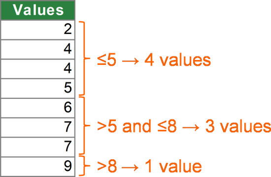
The FREQUENCY formula counts, how often values occur within a range of values. Say you have a set of numeric numbers, for example 2, 4, 4, 5, 6, 7, 7, 9. Now you want to know how many of your number of less than or equal to 5, how many are between 6 and 7 and how many are larger than 8. FREQUENCY counts for each of these three classes the number of values and returns an array containing exactly these three numbers. So the result of the schematic example on the right-hand side would be the array {4,3,1}.
Structure of the FREQUENCY formula

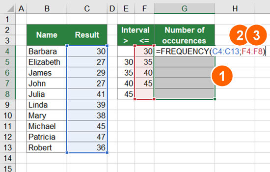
The FREQUENCY formula has two arguments as shown in the image on the right-hand side.
- The “DATA ARRAY” is a range of cells or data which will be―simply speaking―classified into the bins that you specify with the second argument. This argument must be an array of numeric values.
- The “BINS ARRAY” specifies the classes in which the numeric values from the “DATA ARRAY” are grouped. The “BINS ARRAY” must also be numeric values sorted in ascending order.
FREQUENCY is a multi-cell-array formula. That means, in it’s base version it returns an array of values which can be returned to multiple cells. Before you enter the FREQUENCY formula you should select all regarding cells. The results of the formula stretches over the number of cells as the second argument has bins plus one more cell. The reason is that you define the bin borders and you always have one additional bin. Say, you just have one bin (e.g. “5”) then you have the two classes smaller and equal the bin border and larger than the bin border.
Example of the FREQUENCY formula


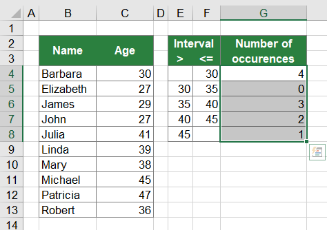
The screenshot on the right-hand side shows a simple example for the FREQUENCY formula. The cell range B4 to C13 contains a list of people and their age in years. You want to know how many people are younger than 30 years old, how many between 35 and 40, and so on. These interval borders are given in cells E4 to F8. The cells G4 to G8 should show the corresponding number of people for each age class. Do the following steps for entering the formula.
- Select all cells that should have a return value. In this example it’s cell G4 to G8.
- Start typing the formula. The “DATA ARRAY” is the age given in cells C4 to C13 and the “BINS ARRAY” is the upper class border in cells F4 to F8.
- Press Ctrl + Shift + Enter on the keyboard.
Please note: Usually you could achieve the same result with the COUNTIFS formula. Because the COUNTIFS formula has some advantages towards FREQUENCY you should consider for such case as in this example to use the COUNTIFS formula. The advantages of COUNTIFS include that it’s more flexible for changes, can be “finetuned” better and is usually faster than an array formula.
Download

Please feel free to download all examples above in this Excel workbook. Click here and the download starts.

