
If the return cell in an Excel formula is empty, Excel by default returns 0 instead. For example cell A1 is blank and linked to by another cell. But what if you want to show the exact return value – for empty cells as well as 0 as return values? This article introduces three different options for dealing with empty return values.
Option 1: Don’t display zero values
Probably the easiest option is to just not display 0 values. You could differentiate if you want to hide all zeroes from the entire worksheet or just from selected cells.
There are three methods of hiding zero values.
- Hide zero values with conditional formatting rules.
- Blind out zeros with a custom number format.
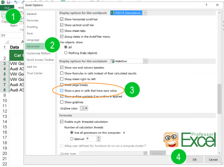
- Hide zero values within the worksheet settings.
For details about all three methods of just hiding zeroes, please refer to this article.

One small advice on my own account: My Excel add-in “Professor Excel Tools” has a built-in Layout Manager. With this, you can apply this formatting easily to a complete Excel workbook.
Give it a try? Click here and the download starts right away.
Option 2: Change zeroes to blank cells
Unlike the first option, the second option changes the output value. No matter if the return value is 0 (zero) or originally a blank cell, the output of the formula is an empty cell. You can achieve this using the IF formula.
Say, your lookup formula looks like this: =VLOOKUP(A3,C:D,2,FALSE) (hereafter referred to by “original formula”). You want to prevent getting a zero even if the return value―found by the VLOOKUP formula in column D―is an empty value. This can be achieved using the IF formula.
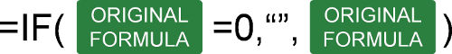
The structure of such IF formula is shown in the image above (if you need assistance with the IF formula, please refer to this article). The original formula is wrapped within the IF formula. The first argument compares if the original formula returns 0. If yes―and that’s the task of the second argument―the formula returns nothing through the double quotation marks. If the orgininal formula within the first argument doesn’t return zero, the last argument returns the real value. This is achieved by the original formula again.
The complete formula looks like this.
=IF(VLOOKUP(A3,C:D,2,FALSE)=0,"",VLOOKUP(A3,C:D,2,FALSE))
Do you want to boost your productivity in Excel?
Get the Professor Excel ribbon!

Add more than 120 great features to Excel!
Option 3: Show zeroes but don’t show blank or empty return values
The previous option two didn’t differentiate between 0 and empty cells in the return cell. If you only want to show empty cells if the return cell found by your lookup formula is empty (and not if the return value really is 0) then you have to slightly alter the formula from option 2 before.
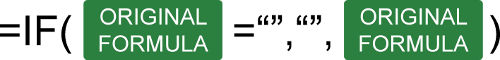
Like before, the IF formula is wrapped around the original formula. But instead of testing if the return value is 0, it tests within the first argument if the return value is blank. This is done by the double quotation marks. The rest of the formula is the as before: With the second argument you define that—if the value from the original formula is blank—the return value is empty too. If not, the last argument defines that you return the desired non-blank value.
The formula in your example from option 2 looks like this.
=IF(VLOOKUP(A3,C:D,2,FALSE)="","",VLOOKUP(A3,C:D,2,FALSE))
Option 4: Use Professor Excel Tools to insert the IF functions very quickly
To save some time, we have included a feature for showing blank cells (instead of zeros) in our Excel add-in Professor Excel Tools.
It’s very simple:
- Select the cells that are supposed to return blanks (instead of zeros).
- Click on the arrow under the “Return Blanks” button on the Professor Excel ribbon and then on either
- Return blanks for zeros and blanks or
- Return zeros for zeros and blanks for blanks.
Professor Excel then inserts the IF function as shown in options 2 and 3 above.

This function is included in our Excel Add-In ‘Professor Excel Tools’
(No sign-up, download starts directly)
More than 35,000 users can’t be wrong.
Option 5: One elegant solution for not returning zero values…
… was written in the comments. Thanks, Dom! Great to get such awesome feedback from you!
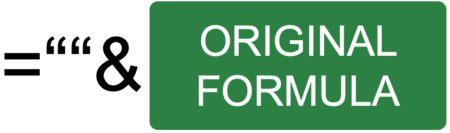
It’s actually quite straight forward: Add two quotation marks in front or after the function and concatenate it with the “&”-character. So, in this case the VLOOKUP function from above would look like this:
=""&VLOOKUP(A3,C:D,2,FALSE)
But: There is a downside. This method forces the cell to a text / string value. This might cause problems in further calculations if a zero is returned. Let me give you an example:
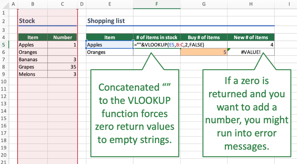
Careful: Return value is interpretated as text.Your VLOOKUP function above is concatenated to an empty string “”. If your return value is 0, the cell will be shown as an empty string. Further calculations might be difficult: For example, if you want to add a number to the return value. Referring directly to the cell, for example =F6+G6 leads to the #VALUE error message as shown above. However, using the SUM function =SUM(F6,G6) still works.
Bottom line: This is an elegant approach, but please test it well if it suits to your Excel model.
Hi Henri can you help me with what is I’m sure a simple problem.
I have text in column A which is one of 4 options. In a related row I have times. I want a function to find the longest time in each text option. An example would be:
A 01:30
B O2:20
A. 02:05
C. 01:31
Etc
Can you help?
Stuart
Options 2 and 3 are seriously ugly solutions. By far the most elegant approach is to concatenate a null string to the lookup result, thus forcing the result to a string:
=””&VLOOKUP(A3,C:D,2,FALSE)
This is the best and most elegant answer I’ve ever seen to this annoying and ongoing problem.
Kudos to you sir!
Thanks, Dom, that’s a great solution. I’ve added it as #4.
Option 3: Show zeroes but don’t show empty return values
sir this formula not working,
show zeros but a same time show the empty return values. please fix this problem
How is Option 3 any different from just using the original formula?
If the value in your original formula is blank, the original formula would (without the if-formula according to number 3) return 0. Using option 3 changes it to blank again.
You can easily try it by just using a cell reference, for example writing =B1 in cell A1. If you leave B1 blank, A1 would show 0. Using the option 3 would show a blank cell A1.
greetings
I have a sumif formula applied to a column that has blanks in it, and in some cases may have ALL blanks. I need to know that when I see a zero it is a ZERO, not a blank being displayed as a zero. I have tried everything.
@Dom: your trick is great, as long as we only need to prevent zeroes to display.
but if I need to do for example
=VLOOKUP(A3,C:D,2,FALSE)<1
cases where VLOOKUP(A3,C:D,2,FALSE) = “” will display TRUE instead of the desired blank value
If we do
=””&VLOOKUP(A3,C:D,2,FALSE)<1, it will always display FALSE whatever the case.
So finally we have no choice but to revert to the – ugly, I concur – suggestion of the article, which is
=IF(VLOOKUP(A3,C:D,2,FALSE)=””;””;VLOOKUP(A3,C:D,2,FALSE)<1)
Thanks for this. Option 3 works great for my database.
Wouldn´t ORIGINAL FORMULA&”” work as well?
That displays the cell as empty if the value is 0
Hi, I am using a simple if statement =IF(G2=”L”,1, ) and I dont want 0 as a false value. I am fine to get a blank cell when False. Please help.
For option 3, Microsoft suggests that you use ISBLANK() function instead of = “”
https://docs.microsoft.com/en-us/office/troubleshoot/excel/use-formula-evaluate-blank-cell
Option 2 worked for me. It’s so simple and useful. Thank you so much!!
Hi Henrik!
I have been using something like this: =If( [condition] , [result if true] , “”)
This formula gives me blanks in case the condition is false and works good for me as it ‘shows’ cells as blanks. But in reality it has some special character which gets copied when I need to. How can I get rid of these special characters in the cell as I will need to keep it like this. Can we use any other option to make it ‘actual’ blank?
Thanks
Mohit
I have the same problem.
When the “” result cell value is copied to another workbook as value it is not empty.
The cell shows as populated and messes up calculations, for example the average of that column is #Value!
It would be better to use some letter instead of “” as it would not interfere down the line.
Hi Henrik,
I’m building a chart and I don’t want empty cells to be plotted.
Using the options for Hidden and Empty Cells in the “Select Data” chart functionality it works .. but only if the cell doesn’t contain a formula.
I tried also using the methods you advise, but anyway the excel charting process plots a “zero” value, because (I guess) it actually finds a formula in the cell (thus the cell is not “empty” or “blank”)
Do you have any tips or workarounds for this issue?
Thanks
Alberto
Hi Alberto,
The trick is to return the error value #N/A. You can you this like this =IF(B5=0,NA(),B5)
Does that help?
Best regards,
Henrik
Hi,
=if(if(N5>J5,N5-J5,T5+0)=0,””,”=if(N5>J5,N5-J5,T5+0)”) this is formula i used, but when the result is not 0 then hpow to get the Correct result here?
Hi beenarani,
Have you tried removing the last two quotation marks and the equal sign?
=if(if(N5>J5,N5-J5,T5+0)=0,””,if(N5>J5,N5-J5,T5+0))
=IF(VLOOKUP(A3,C:D,2,FALSE)=””,””,VLOOKUP(A3,C:D,2,FALSE))
how do i nest this to look up 3 worksheets…
Hi Henrik
My issue is I use a mid & find formula to return a number but when the cell is blank it returns a value sign or name sign, so my question is how to return a cell & leave blank (clear) from the formula below
=MID(D270,FIND(“(“,D270)+1,FIND(“)”,D270)-FIND(“(“,D270)-1)
Regards
Tony
Hi Henrik,
Hope you are doing great. I do have a little bit of problem with my excel formula. The problem is like this.
I want count zeros in a column from subtracting dates without including zeros due to blank cells.
Thanks.
How do I sort tabs in alphabetical order please?
=””& work!! man your genius!
=””& worked!! man your genius!