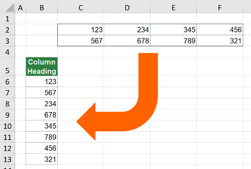
Say, you have an Excel table and want to copy all column underneath each other so that you only have one column. For example, you have a table 2 rows by 4 columns like in the screenshot on the right-hand side. You want to copy and paste this table to one column. You often need such transformation for inserting PivotTables or to create database formats. This article provides 4 simple methods to transform a 2-dimensional table into one column in Excel.
Example
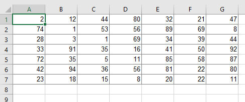
The following methods will be introduced with a simplified example as shown on the right-hand side. You have a table with numbers within the cell range A1 to G7. That means you have 7 rows and also 7 columns. In total 49 cells to be copied to one column.
Method 1: Copy table to one column manually
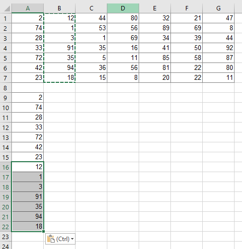
Like so often, copying and pasting the columns manually might be the fastest solution. Given that you are reading this article, this might not be the method you want to hear. But anyway, doing it manually is often the fastest way.
Maybe some advice to speed up the manual process might help. Try to use as many keyboard shortcuts as possible. That way you could save some time.
- Holding Ctrl and pressing one of the arrow keys makes you jump between tables and cells.
- Holding the Shift key, you can select cells and ranges.
- And – of course – with Ctrl + C and Ctrl + V you can copy and paste cells.
For more information about the keyboard shortcuts please refer to our big keyboard shortcut package.
Method 2: The INDEX formula
You can convert a two-dimensional table into just one column by using the INDEX formula. Unfortunately, it requires some preparations. But on the other hand, it’s one of the faster ways (compared to setting up the more complex OFFSET formula like in method 3 below or the INDIRECT formula).
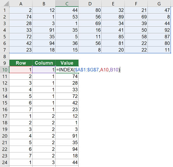
Let’s see what you need to prepare. Basically you have to create the column and row number in additional helper columns. That way you can easily refer to the original table. The screenshot on the right-hand side shows the necessary preparations.
- You need one column containing the row number (here in column A). You always start with 1. So if you data start in row 3, the first number you write is still 1.
- You need one column containing the column number (here in column B). Also for the column number you always start with number one.
- The third column contains the actual values, pulled by the formula =INDEX($A$1:$G$7;A10;B10) . Example: In cell C10, the INDEX formula returns the value from the first row and first column of the range A1 to G7.
Please refer to this article for more information about the INDEX formula in Excel.
Method 3: OFFSET formula
The third method uses the OFFSET formula for copying several columns underneath each other to one column. If you need some introduction to the OFFSET formula, please refer to this article.
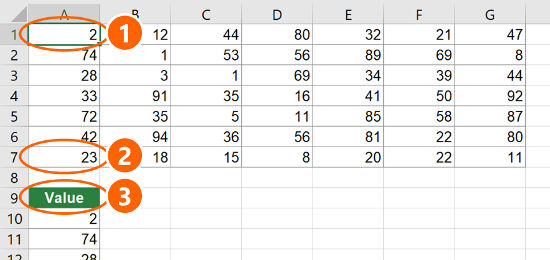
Because the formula is – in this universal case – very long, we don’t go much into detail here. It’s based on three cells.
- The top left cell of the table you want to convert (here: A1).
- The bottom left cell of the table you want to convert (here: A7).
- The heading cell of your single column, which is supposed to contain all the data from the table (here: A9)
Now you just have to replace the cell links in the following formula with your cells. Don’t forget to fix the references with the $-signs as shown in the formula below.
=OFFSET($A$1,(ROW()-ROW($A$9)-1)-(ROW($A$7)-ROW($A$1)+1)*ROUNDDOWN((ROW()-ROW($A$9)-1)/(ROW($A$7)-ROW($A$1)+1),0),ROUNDDOWN((ROW()-ROW($A$9)-1)/(ROW($A$7)-ROW($A$1)+1),0))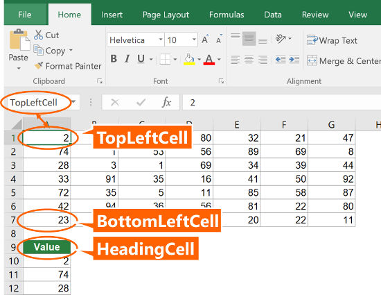
In order to make it easier for you to use the formula, you can use the version below. All you have to do is to give names to the three main cell as shown in the image on the right-hand side. In order to achieve this, select the top left cell of your original table (here: A1) and click into the name field. Type “TopLeftCell” and press Enter on the keyboard. Repeat this with the bottom left cell (name “BottomLeftCell”) as well as the heading cell of your new table (name “HeadingCell”).
Once done, copy and paste the following formula it the first cell (here: A10). Now just copy and paste this cell down until all columns from your original table are covered.
=OFFSET(TopLeftCell,(ROW()-ROW(HeadingCell)-1)-(ROW(BottomLeftCell)-ROW(TopLeftCell)+1)*ROUNDDOWN((ROW()-ROW(HeadingCell)-1)/(ROW(BottomLeftCell)-ROW(TopLeftCell)+1),0),ROUNDDOWN((ROW()-ROW(HeadingCell)-1)/(ROW(BottomLeftCell)-ROW(TopLeftCell)+1),0))Method 4: Professor Excel Tools
You want to use the most convenient way? Try the Excel add-in “Professor Excel Tools”. The steps are shown in the screenshot below.
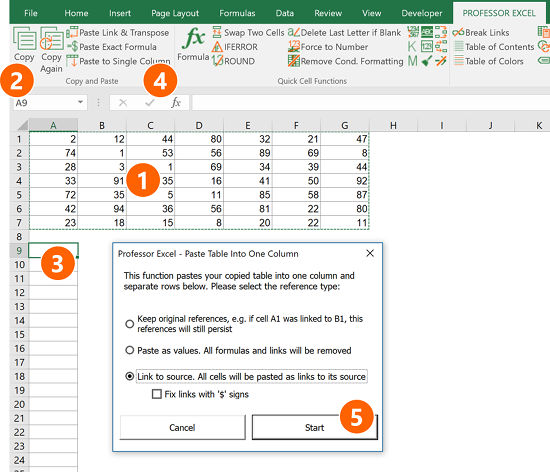
- Select the table you want to transform into a single column.
- Click on Copy on the left-hand side of the “Professor Excel”-ribbon.
- Select the first cell from which Professor Excel should paste the columns underneath.
- Click on “Paste to Single Column” on the “Professor Excel” ribbon.
- Now you can finetune the copy-and-paste-format. Do you which to copy the formulas without changing cell references, do you which to copy them as values or do you want to insert links to the original table? Then press Start.
That’s it. Do you want to try “Professor Excel” for free? Then just follow this link for more information or start the download right away.

This function is included in our Excel Add-In ‘Professor Excel Tools’
(No sign-up, download starts directly)
More than 35,000 users can’t be wrong.
Download
![]() Please feel free to download all examples shown above in one comprehensive Excel file. Just click on this link and the download starts right away.
Please feel free to download all examples shown above in one comprehensive Excel file. Just click on this link and the download starts right away.


The problem can also be solved by inserting helper column “A” with formula:
=IF(ROW()*1/7=INT(ROW()*1/7),ROW()*1/7,INT(ROW()*1/7)+1)
applied downward
and formula:
=INDIRECT(ADDRESS(ROW()-(A8-1)*7,COLUMN()+(A8-1),4))
in cell “B8”, also applied downward.
=OFFSET(TOPLEFT;ROUNDDOWN((ROW()-ROW(HEAD)-1)/(COLUMN(TOPLEFT)-COLUMN(TOPRIGHT)+1);0);-MOD((ROW()-ROW(HEAD)-1);COLUMN(TOPLEFT)-COLUMN(TOPRIGHT)+1))