How to Change Grouping Direction Above / Left of Data in Excel?

Today, I have a quick tip for you: Do you want to change the grouping direction in Excel? Usually when you use groupings on rows, the small + or – sign is below the grouped data. The same for columns: The little + and – sign for showing or hiding grouped columns is located on the right side of the data. But sometimes it’s the other way around, how to change this?

Default grouping position in Excel

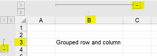
If you add grouping in Excel, the default setting is that the little + and – signs are

• either below the grouped rows or
• to the right of the grouped column.

This is shown in the image above.

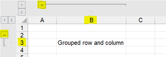
Now you want to change it so that it look like this:

Change the grouping direction to above or left of data

Admittedly, it’s quite hidden:

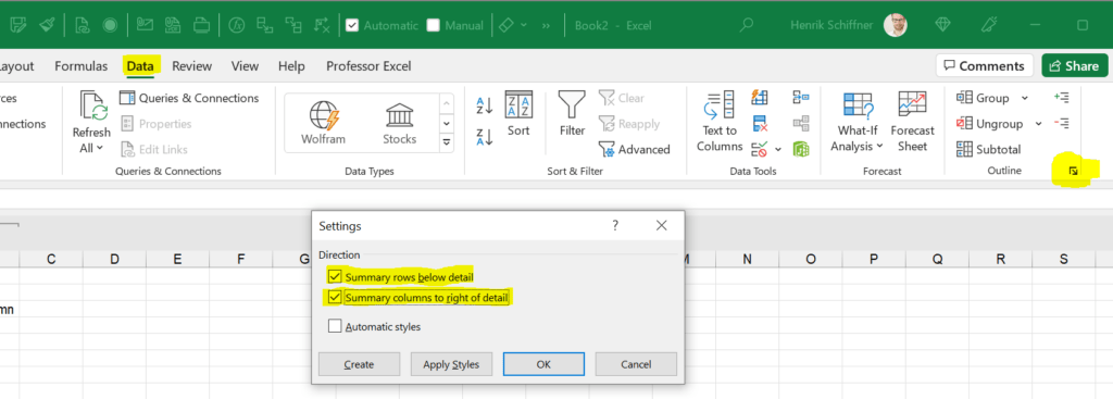
1. Go to the Data ribbon.
2. Click on the tiny arrow in the bottom corner of the outline section.
3. Set the ticks according to your desired direction, for example “Summary rows below detail”.

There is only one disadvantage: You can only set it to one worksheet at a time.

Do it for the whole workbook with Professor Excel Tools

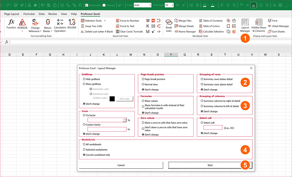
Do you want to do this for several worksheets at the same time? Take a look at our Excel add-in “Professor Excel Tools“. The layout manager provides a function to apply such layout to the complete workbook or just some worksheets.

1. Click on Layout Manager on the Professor Excel ribbon.
2. Select the grouping position of rows…
3. …or of columns.
4. Set the scope: All worksheets, currently selected worksheets or the current worksheet only.
5. Click on Start and the layout is changed immediately.

---

This function is included in our Excel Add-In ‘Professor Excel Tools’

Learn more

Download Free Trial

(No sign-up, download starts directly)

More than 35,000 users can’t be wrong.

---

Image by Eiji Kikuta from Pixabay