You opened an Excel file and it immediately showed an error message saying that there is a circular reference. What to do now? In this article, we’ll learn what are circular references in Excel and how to solve them.
This article is also part of the book “Speeding Up Microsoft Excel“, available on Amazon.
What is a circular reference?
Simply speaking, a circular reference occurs when cell A refers to cell B, and cell B refers to cell A. But often, circular references not only regard two cells, but also follow a long chain of cells. These circular references can slow down the calculation process and more importantly produce wrong results. The basic idea of this method is to avoid circular references in general. If you want to maintain them, then try to use the so-called iterative calculation.
Excel offers two helpful functions concerning circular references. It helps you find circular references, and you can let Excel solve circular references with iterative calculations.
How to find circular references?

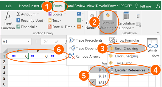
To find circular references, follow these steps to identify and remove them.
- Go to the “Formulas” ribbon.
- If the “Formula Auditing” group is collapsed, as shown in figure 18, then click on it. Otherwise, just continue to step 3.
- Click on “Error Checking.”
- If the “Circular References” button is grayed out such that you cannot click on it, then your workbook has no circular references. If it is not grayed out, then your file has circular references.
- After clicking on the “Circular References” button, you’ll see a list of cells that are involved in the circular reference. This list could potentially contain hundreds of cells.
When you enter a formula that turns out to be part of a circular reference, Excel warns you with an error message. It also shows you the circular reference, with blue arrows pointing out the calculation chain for the circular reference.
How to remove circular references
People often don’t intentionally create circular references; instead, they usually result from formula errors. To remove unintentionally created circular references, you’ll need to correct the corresponding formulas. Here’s a simple example. If cell A refers to cell B, and cell B refers to cell A, then you must break the circle, for example by making cell B refer to cell C instead of cell A.
Alternatively, you can replace one formula cell of the circle by using hard values. Copy and paste one of the cells by using the “Paste Special” dialogue (press Ctrl + Alt + V on the keyboard). Select “Values” and press Enter.
Do you want to boost your productivity in Excel?
Get the Professor Excel ribbon!

Add more than 120 great features to Excel!
Another approach: Iterative calculations

In some cases, you will want to keep the circular references and allow Excel to iterate in order to calculate the result. Excel 2016 allows up to 32,767 iterations. To do this, follow these steps.
- Click on “File” and then “Options.” Navigate to “Formulas,” as shown in figure 19.
- Check the box “Enable iterative calculation.” You can further set the maximum number of iterations as well as the maximum change at which you want Excel to stop iterating. The default value is 100 iterations.
When Excel calculates iterations, you can see the status bar in the bottom-right corner of the screen, which displays the number of the current iteration (for example, “Itr: 1”). In most cases, the maximum number (100 in this case) will not be reached, because the change is smaller than your defined maximum. In practice, if the maximum number of 100 iterations is reached, then the iteration process is stuck and will not yield better results. You can (carefully) reduce the number and see if the results worsen.
But please be careful:
- In many cases, allowing iterative calculations leads to wrong results.
- Iterative calculations can make your workbook very slow.


I set up my worksheet where the dates are auto-populated when an initials is entered. The next day, I put my cursor on the initial field and click on the Save and it automatically change the date to today’s date. As an example I using the following formula:
=IF(BK32″”,IF(AND(BN32″”,CELL(“address”)=ADDRESS(ROW(BK32),COLUMN(BK32))),NOW(),IF(CELL(“address”)ADDRESS(ROW(BK32),COLUMN(BK32)),BN32,NOW())),””)
Also enable the ‘Iterative Calculation’ to automate the date.
Can you please help. Why the date is changing on spreadsheet, when the cursor is left on the initial field after exiting. Please advise.
instead of using now use today, or if you want more granularity us the round formula on now so that it isn’t changing every second.