You are working on an Excel file and have used cell background colors? In such case you might want to insert a legend or table of colors used in your sheet or workbook. Here are three methods that might work for you.
Example in this article
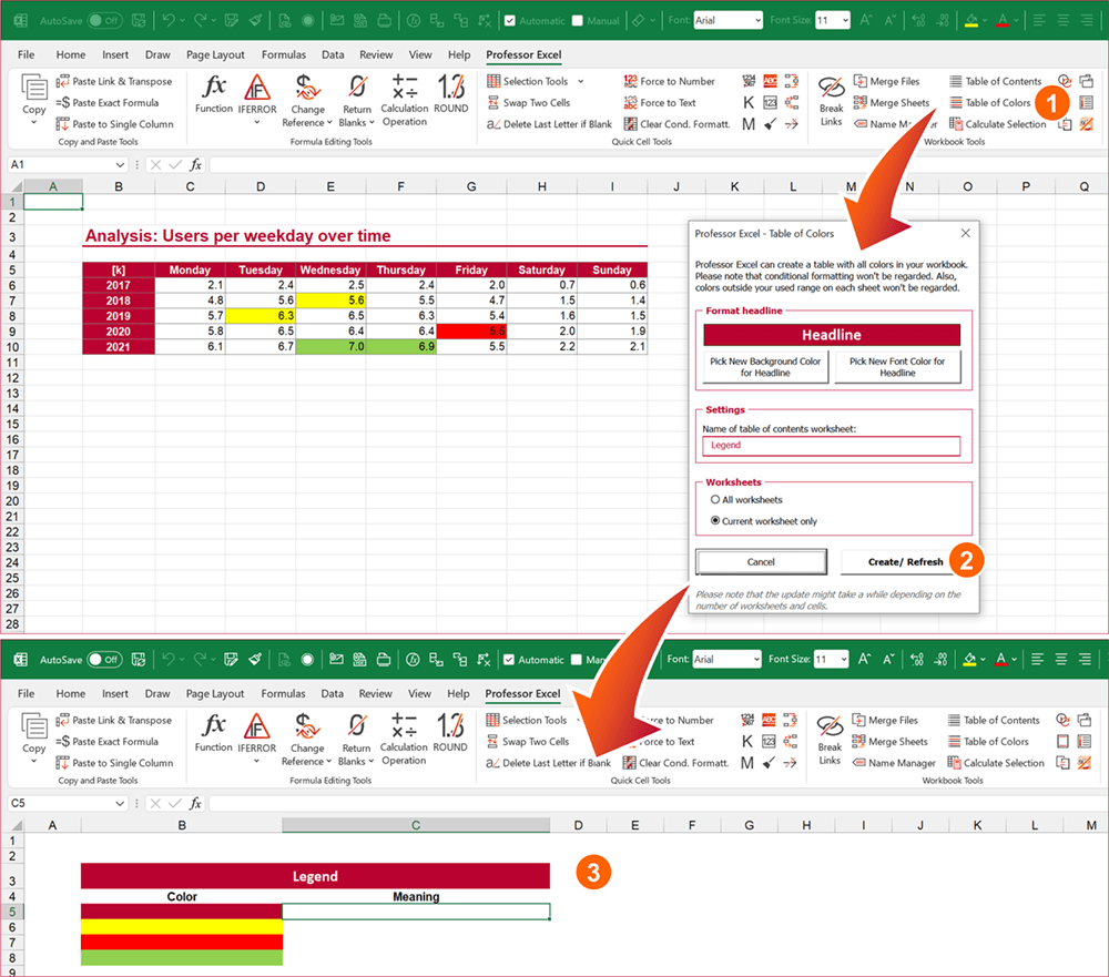
In this article we use the following example. You have created an analysis and highlighted some cells. Now, you want to insert an explanation, primarily for the red, yellow and green cells.

Method 1: Insert a legend manually
Yes, I know, doing things manually is kind of uncool… but often still the fastest method. When it comes to a table of colors, it might be a valid option for you.
When working with colors it is anyway recommended not to use hundreds of different colors. So, usually you would only use up to 5 or 7 different colors, right? If that is the case, try to create a legend manually.
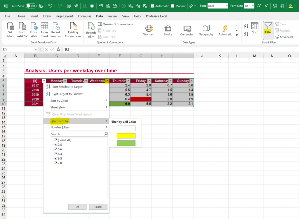
Here is some advice, especially for larger tables than in our example: You can gain an overview of all colors in a column by inserting filters.

- Select the whole range and click on “Filter” on the Data ribbon.
- Then, click on the small filter icon in the heading of a column and scroll down to “Filter by Color”. Now, you can see all different colors used in the column.
Method 2: Use a VBA macro to insert a table of all background colors
Our next method to insert a legend involves a VBA macro. I have prepared a short macro that does the following:
- Insert a new worksheet called “Professor_Excel_Legend”
- On this worksheet, it creates a list of all background colors used on your currently selected
Open the VBA editor window, insert a new module and copy & paste the following code (if you need assistance with these steps, please refer to this article).
Sub createLegend()
    Dim activeSheetName, legendSheetName As String
    activeSheetName = ActiveSheet.Name

    legendSheetName = "Professor_Excel_Legend"
    Sheets.Add
    ActiveSheet.Name = legendSheetName

    Range("B3").Select
    ActiveCell.FormulaR1C1 = "Legend"

    Range("B4").Select
    Dim i, J, currentRow As Integer
    Dim colorFound As Boolean
    i = 0
    currentRow = 4

    Dim cell As Range

    For Each cell In ActiveWorkbook.Sheets(activeSheetName).UsedRange.Cells
        colorFound = False
        For J = 4 To currentRow
            If Sheets(legendSheetName).Cells(J, 2).Interior.Color = cell.Interior.Color Then
                colorFound = True
            End If
        Next
        If colorFound = False Then
            Sheets(legendSheetName).Cells(currentRow, 2).Interior.Color = cell.Interior.Color
            currentRow = currentRow + 1
        End If

    Next cell

End Sub
Method 3: Use an Excel add-in to create a legend comfortably
This method is probably the fastest: Create a legend with an Excel add-in. Our add-in “Professor Excel Tools” comes with many, many features – one of them is “Table of Colors”. It creates a legend either of the current worksheet or a whole workbook at once.

Just click on the “Table of Colors” button on the Professor Excel ribbon. Now, you can specify the settings and click on Refresh / Start. Easy, right?

This function is included in our Excel Add-In ‘Professor Excel Tools’
(No sign-up, download starts directly)
More than 35,000 users can’t be wrong.
Image by Rudy and Peter Skitterians from Pixabay


Very helpful! Thanks!