You’ve probably heard of conditional formatting in Excel, haven’t you? You can format cells based on their values or insert small symbols, also depending on the cell’s values. One advanced scenario of Conditional Formatting is to use formulas to determine the format. For example, you want to change the background color of cell A if cell B has a certain value. Let’s take a look at how to use conditional formatting with formulas.
Steps for using conditional formatting with formulas
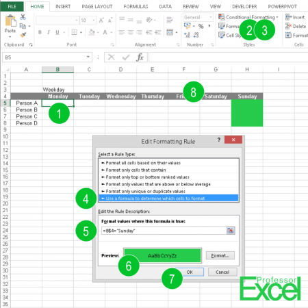
Probably the easiest way of understanding the conditional formatting with formulas is with a specific example. Let’s say, we got a simple timesheet. The columns show weekdays Monday to Sunday and the rows contain different people. Each person has one row. We want to cross out the Sunday for each person by changing the background color (in our case green). How do we do that?
The numbers are corresponding to the picture:
- Select the first cell. In our example it’s cell B5. We are going to apply the conditional formatting for this cell only and copy the formatting to the other cells later on.
- Click on “Conditional Formatting” in the middle of the Home ribbon.
- Click on “New Rule…”
- In the lower dropdown list, choose “Use a formula to determine which cells to format”.
- The condition is quite straightforward: =B$4=”Sunday” . When you copy the cell formatting later on, the column will be adapted, whereas the row always stays the same (row 4).
- Define the format if your condition is true. In our case: red standard formatting.
- Click “OK”.
- Copy cell B5 and paste special the formatting (Ctrl + Alt + v –> t) or use the Format Painter.
That means in conclusion, when the formula returns “TRUE”, the formatting will be applied. Using the $-sign works the same way as in any other formula.
Please note that you can also use complex formulas. But the more complex the formulas get (and the more cells you use them on), this can significantly decrease the performance and your Excel workbook can get very slow.