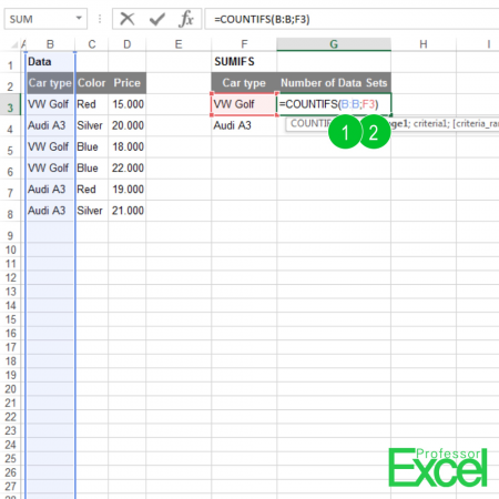
COUNTIFS in Excel: Everything You Need to Know!

COUNTIFS is a very useful formula in Excel: You want to count how many times you got a certain data entry – under several conditions. The COUNTIFS function works similar like the SUMIFS function. But instead of adding up the values, it counts how many items with one or more criteria are in your table.

How to use the COUNTIFS formula

The COUNTIFS formula needs at least two parts: One search range and the criteria you are going to search for. In our example above, we got a column with car brands. You want to know how many times “VW Golf” appears (the numbers are corresponding to the picture above):

1. The column which your criteria is in.
2. The lookup value (in our case “VW Golf”).
3. Optional: Second criteria column.
4. Optional: Second lookup value
5. …

Difference to COUNTIF (without “s”)

COUNTIFS is quite similar to COUNTIF (without “s”). But COUNTIF (without “s”) can only regard one criteria, whereas COUNTIFS can match up to 127 criteria.

Originally, there was only the COUNTIF formula in Excel. Since Excel 2007, Microsoft has added the version with “s” in the end in order to allow more conditions. We recommend only using the COUNTIFS formula, even if you only have one condition. That way, you only have to memorize one formula.

Solve errors with the COUNTIFS formula

• You got a wrong result, for example the returning number is not as expected?
  • Make sure that all criteria ranges have the same size, for instance, column A1:A5 and B1:B5
  • Are all criterias formatted correctly, e.g. numbers as numbers and text cells as text?
• You get a 0 (zero) returned, although there should be another value? Most probably, the search criteria don’t match.
• For other errors, please check out the error helper. Select your error message in the upper box and COUNTIFS in the lower one. Press ‘Solve error’ to receive more information about the error and in combination with COUNTIFS.

Special case 1: COUNTIFS horizontally

Our first special case is using the COUNTIFS formula horizontally. The search and condition ranges have a horizontal shape. The formula itself works exactly the same way like the vertical version.

You got the table with car type as shown in the image above. Now you want to count in column M, how often you got each car and color combination in your data.

=COUNTIFS($B$2:$I$2,K3,$B$3:$I$3,L3) 

Let’s go through it step by step:

1. The first part ($B$2:$I$2) contains the condition range of the car type. The dollar signs fix this range as you will later on copy the formula.
2. The second part (K3) is the first car type – in this case “VW Golf”. This cell is not fixed with dollar signs, as you want it to change when you copy and paste the formula.
3. The third part ($B$3:$I$3) contains the condition of the car color. Again, this range is fixed with the dollar signs.
4. The last part (L3) is the color, in this case “Red”.

Special case 2: Criteria with larger or smaller

In our next example we want to count list entries with greater and smaller than certain values. In this case: We want to know, how many case there are under 17,000 EUR, between 17,000 and 20,000 EUR and above 20,000 EUR.

The trick: add “>”& and “<=”& to the formula. The complete formula in cell F3 looks like this:

=COUNTIFS($B$3:$B$10,">"&D3,$B$3:$B$10,"<="&E3)

Again, let’s take a look at each part individually:

1. The first condition range is the price, in this case given in range B3 to B10.
2. The first condition: We want to know the number of items larger than 0 (cell D3).
3. The second condition range is again the price.
4. The second condition: Similar to the first condition we want to know all items also smaller than 17,000 (cell E3).