SUBTOTAL in Excel: Everything You Need to Know – Big Guide!

SUBTOTAL is one of those formulas in Excel, which is very powerful but not well known. The reason is, that you can achieve all its operations by other formulas as well. But in many cases, SUBTOTAL would be the better choice. Read here how to use it and why SUBTOTAL is very useful.

Structure

The short description of SUBTOTAL in Excel is quite vage:

Returns a subtotal in a list or database

In order to be more specific: The SUBTOTAL formula can perform a mathematical calculation to one or more cell ranges. Instead of only being able to perform one fixed operation, you can choose the calculation type (e.g. sum, count, average) as an input variable. Furthermore, the SUBTOTAL formula has some more great advantages towards the distinct formulas.

Arguments

The SUBTOTAL formula has (at least) two parts. The function type as well as the cell reference. Why “at least”? Because you can add up to 254 cell references.

The arguments of the SUBTOTAL formula are shown above:

1. The first argument of the SUBTOTAL formula is the function number. With this function number you determine the operation of the formula. E.g. if you want to add up value, just type 9. Or if you want Excel to count for you type 2. Please scroll down to the section “function types” in order to see all available operations.
2. The cell reference containing the values you want to calculate with. This argument is – like the function number – compulsory.
3. Starting here all arguments are optional. Excel allows you to select up to 254 cell references you want to include in your calculation, separated by commas.

Function types​

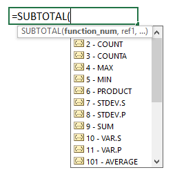
There are 11 different operations you can use with the SUBTOTAL function. They are numbered by values from 1 to 11. You can use each of those functions types in two different ways:

1. Regard all cells given in the cell references. No matter if they are hidden, shown or grouped. For selecting such operation use the function number 1 to 11.
2. Only the visible cells. So if you hide rows or columns in between, they won’t be regarded. For using such operation use the corresponding function number 101 to 111.

All available functions are summarized in the table below. But don’t worry, you don’t have to remember all of them. When you start typing =SUBTOTAL( into an Excel cell, Excel will provide a list of available functions with their numbers.

Function	Description	# for all cells in range	# for only visible cells in range
AVERAGE	Returns the arithmetic mean	1	101
COUNT	Returns the number of cells in range that countain numbers	2	102
COUNTA	Returns the number of cells in range that are not empty	3	103
MAX	Returns the largest value	4	104
MIN	Returns the smallest value	5	105
PRODUCT	Multiplies all values	6	106
STDEV.S	Estimates the standard deviation based on a sample	7	107
STDEV.P	Calculates the standard deviation of all numbers	8	108
SUM	Adds all the numbers	9	109
VAR.S	Estimates the variance based on a sample	10	110
VAR.P	Calculates the variance of all numbers	11	111

Important: Characteristics of the SUBTOTAL formula

Now we are getting to the interesting part. It will also explain why should you use SUBTOTAL. So far everything we know is also covered by easier formulas. For example =SUM() also adds up values.

• SUBTOTAL disregards results of other SUBTOTAL formulas. This is very important because if you want to insert results in between a longer calculation chain, you could easily do so without adjusting to total result. For more information scroll down to “Example 2”.
• You can ignore hidden values. This can be useful if you got a sheet full of filtered data and you instantly want to know the number of rows or the displayed sum.
  It can ignore the following values if you choose the function types >100:
  • Hidden rows.
  • Grouped/ outlined rows.
  • Filtered rows.

    But: SUBTOTAL does not ignore hidden columns! Only rows.

• SUBTOTAL can only use 2-dimensional ranges. If you try to use SUBTOTAL on a 3-dimensional cell range, e.g. B3:C5, it returns a #VALUE error.

Example 1: The basics

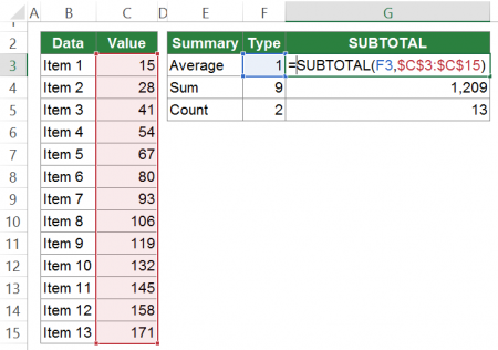
Let’s jump right in with an example after so much theoretical knowledge.

You got some data in column B and C. Now you want to use the SUBTOTAL formula for summarizing it in the table on the right side. You want to get the following functions:

• The average of the values,
• the sum and
• the number of items in the list.

The SUBTOTAL formula for the average is quite simple: =SUBTOTAL(1,”CELL RANGE”) . Instead of just typing “1” as the first argument, you can also link to the cell defining the operation. In this case the function number if given in column F so you just link to cell F3.

The second argument is the cell range. In this example it’s the range C3 to C15. In order to fix the cell range you can add the $ signs. When you copy the formula into the cells G4 and G5, this range will persist. Combining these two arguments, the complete formula is =SUBTOTAL(F3,$C$3:$C$15)  .

Expert tip: Let Excel do the work for you

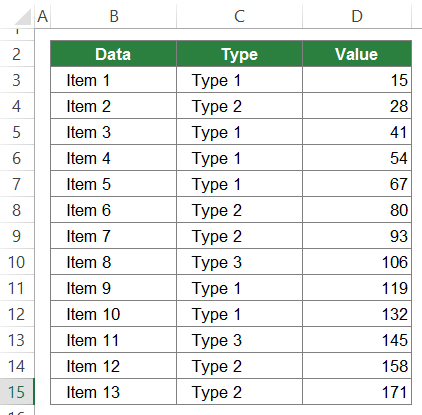
Excel can help you to insert the SUBTOTAL function. All you need: Your data must be in a database format. That means the format has to be similar to when you insert a PivotTable. Please refer to this article for more information about how to achieve such data structure.

Step 1: Organize your data

Let’s say you got the data as shown in the image on the right side. It contains a short description in column B, a data type and a value. You want to organize and summarize your table by the data type in column C.

The first step: Sort the data. If you want to summarize the table by the type in column C, you have to sort it by column C. The reason for that: Excel adds a new column with a SUBTOTAL formula under each change of type.

Step 2: Find the SUBTOTAL function

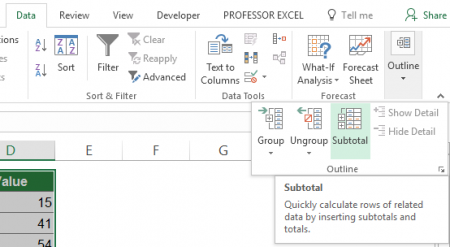
Once your data is sorted, select the complete table and click “Subtotal” within the Outline groups. It’s located on the right side of the Data ribbon.

Step 3: Define the SUBTOTAL settings

Now you see a new windows which looks like the one on the right. It basically has 5 sections:

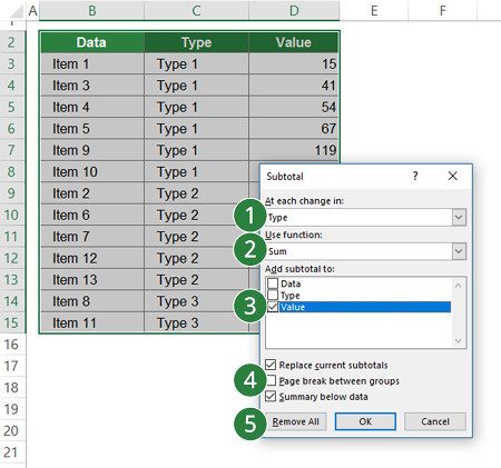
1. Excel needs to know for which rows you want to insert the SUBTOTAL function. It will add new rows between each change of this field.
   In your case you want to summarize the values each time the type changes. So please select “Type” (column C) here.
2. Which function do you want to use? Probably in most cases you want to add up the values – so please select “sum”.
3. Where are your numeric values located? In this example it’s the column D, called “Values”.
4. You can further specify:
   1. Let’s assume you already got SUBTOTALS within your table. In such case: Do you want to replace current SUBTOTALS? Or do you want to add one more layer of SUBTOTALS to existing ones?
   2. Excel can add page breaks. This is rather a layout option and might be relevant to you when you work with large sets of data.
   3. Do you want to get a summary row under the whole table?
5. Of course, you can also let Excel remove existing SUBTOTAL structure. In that case click “Remove all”.

The result

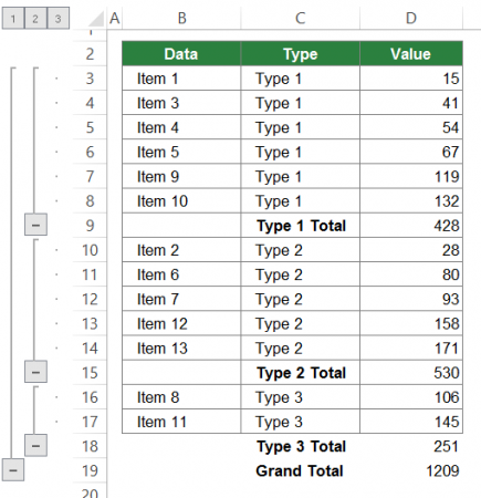
Click “OK”. The result of the SUBTOTAL structure looks like on the right side. Excel not only inserts the SUBTOTAL rows. It also provides the matching outline structure.

The formula in cell D9 is: =SUBTOTAL(9,D3:D8) and the formula in cell D19 (the Grand Totals): =SUBTOTAL(9,D3:D17) .

If you want to summarize your table by one more criteria, repeat these steps. But make sure you don’t set the tickmarks at “Replace the current subtotals”.

Example 2: Ignore all other SUBTOTALs

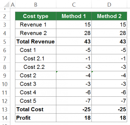
In many cases, your Excel table has some “level” structure: You got a lot of rows containing data. In between you got sums and those sums in return add up to a total. That could be the case for a balance sheet or P&L statements (see the picture).

You got two options for getting such table:

1. Using distinct formulas and link directly to the cells. This method is shown in column C. The problem with this method: You have to be very careful not to “forget” any value and make sure that all your references are intact.
2. The other way would be with the SUBTOTAL formula. As described above, the Method 2 using SUBTOTALS has an advantage: It ignores other SUBTOTALs. So the formula in your Grand Total can stretch over the complete range if your sums in between are also using SUBTOTAL.

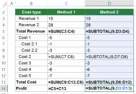
If you take a look at the formulas of Method 1 you will see, that it takes some care to apply them. You really have to be cautious to get link the sums and “+”-operations to the correct cells. It might be fine in this example because you only have 10 rows. But in reality such tables are much longer.

In contrast the Grand Total (here: Profit) of Method 2 can comfortably stretch over the complete cell range. Furthermore, you can be sure that all input values are regarded once.

Example 3: Only regard visible cells

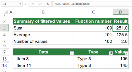
There is another common usage for SUBTOTAL: Get quick results from large sets of data. Typically the formula is above your actual data. Depending on what you select in your database below, the SUBTOTAL formula always shows the result of the current selection.

For such application, you Excel provides the function types 101 to 111 of the SUBTOTAL formula. Please take a look at the picture on the right side. The upper cells (range B2 to D5) contain the summary with the SUBTOTAL formulas. The lower cell range (B7 to D20) contain the data with filters.

The filter in column C (cell C7) is set to “Type 3”. Only two rows are shown. The summary block above has the result of the visible values in column D. You can easily use the SUBTOTAL formula. It has only two parts:

1. Function number: In cell D3 you want to return the currently visible sum. Therefore type 109. Alternatively link to a cell saying “109” – in this case cell C3.
2. The cell range containing your numeric values. In this case its D8 to D20. As you next want to copy and paste the formula and want to keep the cell range, you can add the $-signs.

The complete formula looks like this: =SUBTOTAL(C3,$D$8:D$D$20)

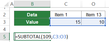
Please note: This only works on hidden rows. If you hide or group columns, SUBTOTAL will regard also hidden cell. Please take a look at the example on the right side. If only visible cells are regarded, this formula would return 25. But SUBTOTAL does not disregard hidden columns. Therefore, the result is not 25 but also includes the values in the hidden columns D to N.

Conclusion of SUBTOTAL

SUBTOTAL is very useful in the following cases:

• You got a calculation within different levels.
• Your calculation type changes depending on an input variable.
• You only want to regard cells in visible rows.

Excel even helps you applying SUBTOTALs to your data. Unfortunately, SUBTOTAL is not very known. The reason: All of it’s functions can somehow (less comfortably) achieved by other formulas. But once integrated in your daily worklife, it can be a great help.

Please feel free to download all the examples above in one Excel workbook.