Table of Contents in Excel: 4 Ways to Create a Directory

Table of Contents in Excel: 4 Ways to Create a Directory

posted on 19 Mar 16

comments 15

Sometimes Excel workbooks become quite large: The more worksheets there are, the more difficult it is to keep the overview. A table of contents might help. In this article we’ll explore 4 ways of creating tables of contents in an Excel workbook.

Let’s say we want to create a new worksheet with a list of all other worksheets. Furthermore, each list entry should have a link to the corresponding worksheet so that you can easily click on it and will be taken to this worksheet at once. Basically, there are four methods for creating such table of contents: Do it manually, apply a complex formula, use a VBA macro or an Excel add-in.

Contents

Method 1: Create a table of contents manually
Method 2: Use formulas for a table of contents
Method 3: Use a VBA macro to create a table of contents
Method 4: Use an Excel add-in to create a table of contents

Method 1: Create a table of contents manually

Insert a table a contents manually

The first method is the most obvious one: Type (or copy and paste) each sheet name and add links to the cells. These are the necessary steps:

Create a new worksheet by right clicking on any worksheet name and click on Insert Sheet (or press Shift + Alt + F1). Give a proper name, for example ‘Contents’.
Start by typing the first worksheet name into cell B4 (or any cell you like…).
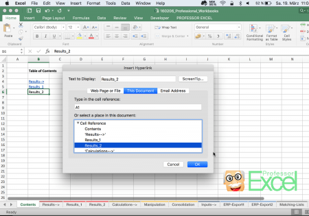
Add the link to the cell: Right click on the cell and click on ‘Hyperlink’. Select ‘This document’ as shown on the picture above and click on the sheet name you want to create the list entry for. Usually cell A1 is fine as the cell reference. The window of adding a hyperlink on Windows looks a little bit different but offers the same options.
Repeat steps 2 and 3 until all worksheets are in your table of contents.
Do all the formatting as desired and then you are done.

Method 2: Use formulas for a table of contents

Define a named range first in order to insert a table of contents with formulas.

Thanks to Brian Canes, who posted this method as a comment: There is actually a way of using formulas and named ranges. Follow these steps:

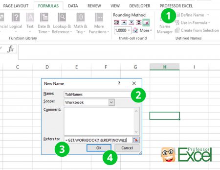
Click on “Define Name” in the center of the Formulas ribbon.
Type the name “TabNames”.
Copy and paste this code into the “Refers to:” field: =GET.WORKBOOK(1)&REPT(NOW(),)
Confirm with OK.
Copy this formula down.

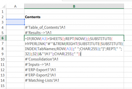
Copy this formula into any cell. As it refers to the cell A1, it’ll be the entry for the first worksheet in your workbook: =IF(ROW(A1)>SHEETS(),REPT(NOW(),),SUBSTITUTE(HYPERLINK("#'"&TRIM(RIGHT(SUBSTITUTE(SUBSTITUTE(INDEX(TabNames,ROW(A1))," ",CHAR(255)),"]",REPT(" ",32)),32))&"'!A1",TRIM(RIGHT(SUBSTITUTE(SUBSTITUTE(INDEX(TabNames,ROW(A1))," ",CHAR(255)),"]",REPT(" ",32)),32))),CHAR(255)," "))
Copy this formula down until you get blank cells.

Please note:

All worksheets will be regarded, also hidden ones.
If you change the order of worksheets, delete some or do any other changes: These changes will be immediately reflected in the table of contents. So you have to be careful if you add comments or do any special formatting.
You have to save the workbook as a macro enabled workbook in the format “.xlsm”. The reason is that you use a formula as a named range which is only possible with macro-enabled workbooks.

Excel too slow? Speed it up. Get the book now!

Table of Contents in Excel: 4 Ways to Create a Directory

Tired of waiting for Excel? Use the 30 best methods described in this book to speed up Excel calculations!

Learn how Microsoft Excel performs calculations
Use the simple and effective step-by-step guide to master each method
Get to know the impact each method will have on performance

Learn more or get it on Amazon!

Method 3: Use a VBA macro to create a table of contents

As the first method works but is quite troublesome – especially for large workbooks – we’ll take a look at a second method: A VBA macro. The macro is supposed to do the same steps: Walk through all sheets, create a list entry for each sheet and insert a hyperlink to each sheet.

Go to the developer ribbon.
Click on “Editor”.
Add a new module.
Paste the following code.
Press start on the top.

Sub insertTableOfContents()
    Dim PROFEXWorksheet As Worksheet
    Dim tempWorksheetName, tempLink, nameOfTableOfContentsWorksheet As String
    Dim i As Integer
    
    'Add a new worksheet
    Sheets.Add

    'Rename the worksheet
    nameOfTableOfContentsWorksheet = "TableOfContents"
    ActiveSheet.Name = nameOfTableOfContentsWorksheet

    'Add the headline
    Range("B3") = nameOfTableOfContentsWorksheet

    'Initialize the counting variable i
    i = 0
    
    
    'Go through all worksheets as described
    For Each PROFEXWorksheet In Worksheets
            'Copy the current worksheet name
            tempWorksheetName = PROFEXWorksheet.Name

            'Create the link from the current worksheet and link it to cell A1
            tempLink = "'" & tempWorksheetName & "'!R1C1"
            
            'Add the list entry
            Sheets(nameOfTableOfContentsWorksheet).Cells(i + 5, 2) = tempWorksheetName

            'Select it for inserting the hyperlink
            Sheets(nameOfTableOfContentsWorksheet).Cells(i + 5, 2).Select

            'Insert the hyperlink
            ActiveSheet.Hyperlinks.Add Anchor:=Selection, Address:="", SubAddress:=tempLink

            'Proceed with next entry and increase i therefore
            i = i + 1
    Next
End Sub

Sub insertTableOfContents()

Dim PROFEXWorksheet As Worksheet

Dim tempWorksheetName, tempLink, nameOfTableOfContentsWorksheet As String

Dim i As Integer

'Add a new worksheet

Sheets.Add

'Rename the worksheet

nameOfTableOfContentsWorksheet = "TableOfContents"

ActiveSheet.Name = nameOfTableOfContentsWorksheet

'Add the headline

Range("B3") = nameOfTableOfContentsWorksheet

'Initialize the counting variable i

i = 0

'Go through all worksheets as described

For Each PROFEXWorksheet In Worksheets

'Copy the current worksheet name

tempWorksheetName = PROFEXWorksheet.Name

'Create the link from the current worksheet and link it to cell A1

tempLink = "'" & tempWorksheetName & "'!R1C1"

'Add the list entry

Sheets(nameOfTableOfContentsWorksheet).Cells(i + 5, 2) = tempWorksheetName

'Select it for inserting the hyperlink

Sheets(nameOfTableOfContentsWorksheet).Cells(i + 5, 2).Select

'Insert the hyperlink

ActiveSheet.Hyperlinks.Add Anchor:=Selection, Address:="", SubAddress:=tempLink

'Proceed with next entry and increase i therefore

i = i + 1

End Sub

Method 4: Use an Excel add-in to create a table of contents

table, of, contents, add-in, professor, excel, tools, table of contents, directory, index

Insert a customized table of contents with the Excel add-in ‘Professor Excel Tools’

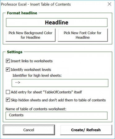
There are some Excel add-ins for creating a table of contents. We – of course – recommend our own add-in. It doesn’t only insert a table of contents but you can easily customize it:

You can customize the headline color.
You can choose if you want to insert links to each worksheet.
You can define levels: For example by high level sheets by their name.
You can select if you want to insert an entry for the table of contents sheet itself.
You can choose if you want to skip hidden worksheets or include them as well.
You can define your preferred name for the table of contents sheets.

Your last settings will be saved so that it’s very fast to update or create a table of contents. There is a 31-day free trial version with no sign-up available. You can just give it a try.

This function is included in our Excel Add-In 'Professor Excel Tools'

Learn more Download Free Trial
(No sign-up, download starts directly)
More than 10k people on Facebook can't be wrong.

Henrik Schiffner

Henrik Schiffner is a freelance business consultant and software developer. He lives and works in Hamburg, Germany. Besides being an Excel enthusiast he loves photography and sports.

Comments 15

Brian Canes

August 21, 2016 • Reply

Here is a way with an Excel4 defined name and a couple cell formulae.
Define TabNames=GET.WORKBOOK(1)&REPT(NOW(),)
In a cell enter the following formula
=”B O O K = “&TabNames&” “&” S H E E T S = “&SHEETS()
In the cell below that enter the following formula
=IF(ROW(A2)>SHEETS(),REPT(NOW(),),SUBSTITUTE(HYPERLINK(“#'”&TRIM(RIGHT(SUBSTITUTE(SUBSTITUTE(INDEX(TabNames,ROW(A2)),” “,CHAR(255)),”]”,REPT(” “,32)),32))&”‘!A1″),CHAR(255),” “))
and fill down until you get empties.
Regards
Brian

Loading...
- Henrik Schiffner
  
  August 22, 2016 • Reply
  
  Dear Brian,
  Thanks a lot, that’s a good way! I’ll add it.
  Best regards,
  Henrik
  
  Loading...
Hayden

May 24, 2017 • Reply

Is there a way with Method 2 of then being able to hyperlink back from the sheets to the table of contents. That would be amazing.

Loading...
- Henrik Schiffner
  
  May 29, 2017 • Reply
  
  Dear Hayden,
  
  There are two simple approaches.
  
  If you are sure that – let’s say – cell A1 is unused on each sheet, prepare a link to the table of contents in cell A1 on one of the sheets.
  In order to achieve this, select the cell and press Ctrl + K on the keyboard. In the “Insert Hyperlink” window select “Place in This Document” and define the link to the table of contents. Confirm with OK.
  Copy the cell and select all worksheets which should link to the table of contents. Paste the copied cell with Ctrl + v. Now, each worksheet should have a link to the table of contents.
  
  Alternatively prepare a text box, also linking to the table of contents sheets (similar to the first method above). Copy it and paste it on each worksheet separately.
  
  Does that help?
  
  Best regards,
  Henrik
  
  Loading...
nhetnai

May 26, 2017 • Reply

For a faster way to create a table of contents, see Create a table of contents automatically.

Loading...
Ralse

June 7, 2017 • Reply

The VBA only seems to work just once and gives an error on ‘already existing name for sheet’ when used again.
Method 2 is more durable for end users unless method 3 refreshes itself when a new sheet is added.

Loading...
i4laughlin.com

June 16, 2017 • Reply

Repeat steps 3 and 4 for all the levels that you want to display in your table of contents.

Loading...
Craig Seifferth

June 6, 2018 • Reply

I tried Method 2: Use formulas for a table of contents multiple times and when pasting the second, longer formula that begins with

=IF(ROW(A1)>SHEETS(),REPT(NOW . . . .

all I get is this error in the cell: #NAME?

Any suggestions?

Loading...
- Henrik Schiffner
  
  June 16, 2018 • Reply
  
  Hi Craig,
  For me the method worked so I can’t really reproduce the error. But the #NAME error usually indicates – as the word says – a problem with a name. And because this method uses a named range, maybe there is a problem? Also have you checked if you’ve spelled all formula names correctly?
  Best regards,
  Henrik
  
  Loading...
kyle andrei mazon

June 15, 2018 • Reply

i know this already…… but i learn some ideas in order to work fast…….!!!

Loading...
Tomasz

January 25, 2019 • Reply

Dear Henrik,

thank you very much for Method 3.
I have a question :
i was trying to make such TOC for sheets which are visible.
In excel file I have about 30 sheets, but depends from case I choose, for printing I have only 7-10 visible.

If I use method 3 then all sheets (about 30) are taken for TOC, but I would like to have only visible.
I’m not expert in VBA, I was trying to play with parameter .Visible but it doesn’t work.
If you can give some tip I will be very grateful.

Best Regards,
Tomasz.

Loading...
- Henrik Schiffner
  
  January 25, 2019 • Reply
  
  Hi Tomasz,
  Without trying it: You could add something like
  
  If PROFEXWorksheet.Visible = True Then
  
  after
  
  For Each PROFEXWorksheet In Worksheets
  
  and
  
  End If
  
  before
  
  Next
  
  Does that work?
  
  Best regards,
  Henrik
  
  Loading...
- Henrik Schiffner
  
  January 25, 2019 • Reply
  
  …and of course my add-in provides this functionality… 😉
  
  Loading...
Kgashane

February 12, 2019 • Reply

Hi Henrik

Thanks a lot for this. How do I get it to list the contents of Cell A1 of each tab, instead of the tab name?

Loading...
chris

March 15, 2019 • Reply

any formula to show the page number?

Loading...