
One of the most often used functions when creating an Excel model is consolidating data from different sources. Traditionally, there were 3 major functions for combining data from different tables or worksheets: VLOOKUP, SUMIFS and INDEX/MATCH. Now, Microsoft has introduced XLOOKUP. So what is the difference between these four lookup functions and which one should you use?
This article was updated in September 2021 for regarding the new XLOOKUP function in Excel. For more information about the XLOOKUP function, please refer to this article.
Overview of the four lookup functions
Let’s take a look at each of the four functions separately, before we eventually compare them and see, which one of them to use in what case.
VLOOKUP
VLOOKUP is probably the best known formula for getting data from another table. The application is fairly easy, although there are some common mistakes which people tend to make. The VLOOKUP formula has four parts (“arguments”):
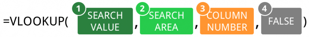
- The lookup value.
- The range, where you are going to search in (Excel searches in the left-most column from this range).
- The number of column, which you want to be returned (start counting from the left column of the search range).
- One optional value, which you can always consider to be “FALSE”
Make sure that you don’t make the most common mistakes as having a too small range (search column as well as return column must be within the search range) and start counting the search column as column number 1.
For more information, please refer to this article.
SUMIFS
SUMIFS only exists since Excel 2007 and is especially useful, as it can regard several search criteria. Also, this application is quite straightforward:
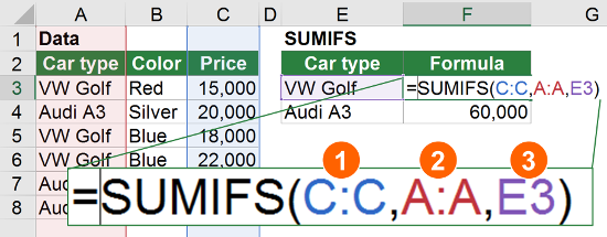
- The column, which the return value is in
- The column, which your criteria is in
- The lookup value
- Optional: Second criteria column
- Optional: Second lookup value
- …
The primary function of SUMIFS is to sum up values matching your criteria. In our case, we must make sure that each criteria combination only exists once in our table. In the example on the right hand side, we would have exactly this problem: There are 3 VW Golfs in our table, so the return value is the sum of the 3 prices.
Please check this article for more information.
INDEX/MATCH
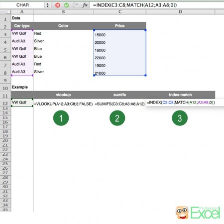
A combination of the two functions index and match has one more advantage than the VLOOKUP: It returns the value from any column and not just on the right hand side of the search column. That usually makes it more stable, because the return column stays the same if you insert more columns in-between.
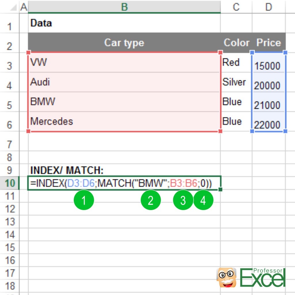
The INDEX formula returns the n-th value from an array of cells. With MATCH, you can search for a value within an array of cells and it’ll return the number of the first occurrence. Please refer to number 3 in above picture for an example of how to use it.
For more information about how to use INDEX/MATCH please refer to this article.
XLOOKUP
XLOOKUP is the newest addition to the lookup functions in Excel. It solves many problems of VLOOKUP and even INDEX/MATCH. At the same time, it’s comparatively easy to use. Here is the basic structure:

The first three arguments are quite straight forward – the arguments 4 to 6 are optional.
- Search value: What do you look for?
- Search area: Where to you look (for example a column or row)?
- Return area: Where is the return value, can also be a column or row (but should have the same shape as the search area.
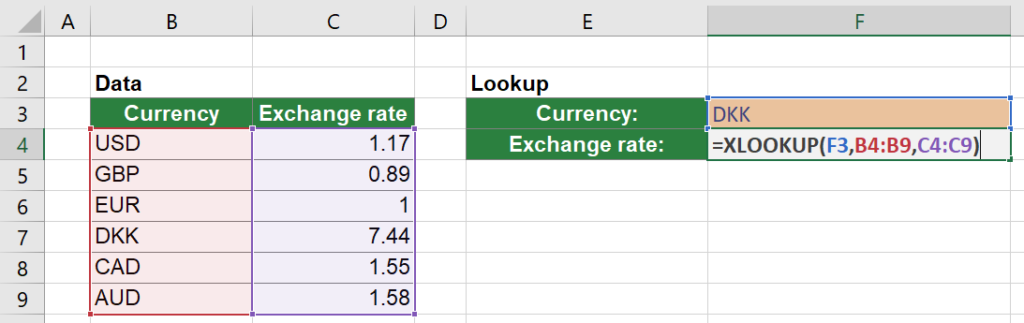
Here is a simple XLOOKUP example:
I won’t go further into detail here. If you want to know more about XLOOKUP, please refer to this article for the basic usage and this article for advanced examples, including the arguments 4 to 6.
Comparison of the lookup functions VLOOKUP, SUMIFS, INDEX/MATCH and XLOOKUP
In the below you can find a comparison of the four functions.
| Criteria | VLOOKUP | SUMIFS | INDEX/MATCH | XLOOKUP |
|---|---|---|---|---|
| Application | Medium | Easy | Difficult | Easy |
| Return numbers | Yes | Yes | Yes | Yes |
| Return texts | Yes | No | Yes | Yes |
| Return column | Only to the right of the search column | Any | Any | Any |
| Lookup values exist multiple times | Return first instance | Return sum | Return first instance | Return first or last instance |
| Stability1 | Low | High | High | High |
| More than one search criteria | No | Yes | No | No |
| Comment | Well known among Excel users | Very versatile, can be used for 2D or 3D lookups | Very versatile |
- XLOOKUP and SUMIFS can be applied rather easily, whereas the INDEX/MATCH combination is – at least for beginners – more difficult.
- All of the lookup functions can return numbers as their return value.
- Unfortunately, SUMIFS cannot return a text as the return value. That means, if you need to return a text, SUMIFS is out of the game.
- The return column for the VLOOKUP must be on the right hand side of the search column. Of course, there are workarounds: Changing the order of the columns or duplicating the return column. There is even an array version of VLOOKUP, but this is quite complicated and not recommended.
- VLOOKUP as well as INDEX/MATCH return the value first in the list. If your search value appears a second time, the second occurrence won’t be regarded. SUMIFS returns the sum. XLOOKUP, however, can return either the first value found (default) or the last.
- XLOOKUP, SUMIFS and INDEX/MATCH are rather stable, as they will still work if you change any column order or delete/ insert columns.
- SUMIFS is the only of the four lookup functions, which can by default regard several search criteria. If you want to search for more than one criteria with one of the other two functions the best way would be to insert a column with a ‘primary key’. This key combines all the search columns into one column. You then only search within this column.
Do you want to boost your productivity in Excel?
Get the Professor Excel ribbon!

Add more than 120 great features to Excel!
When to use which of the lookup functions
Situation 1: Not everyone around you has access to newer Excel versions and therefore cannot use XLOOKUP
First question: Do you and your co-workers / clients etc. have newer Excel versions (Microsoft 365). If you are not sure, it’s probably not the right time to use XLOOKUP yet. In such case, follow this decision tree:
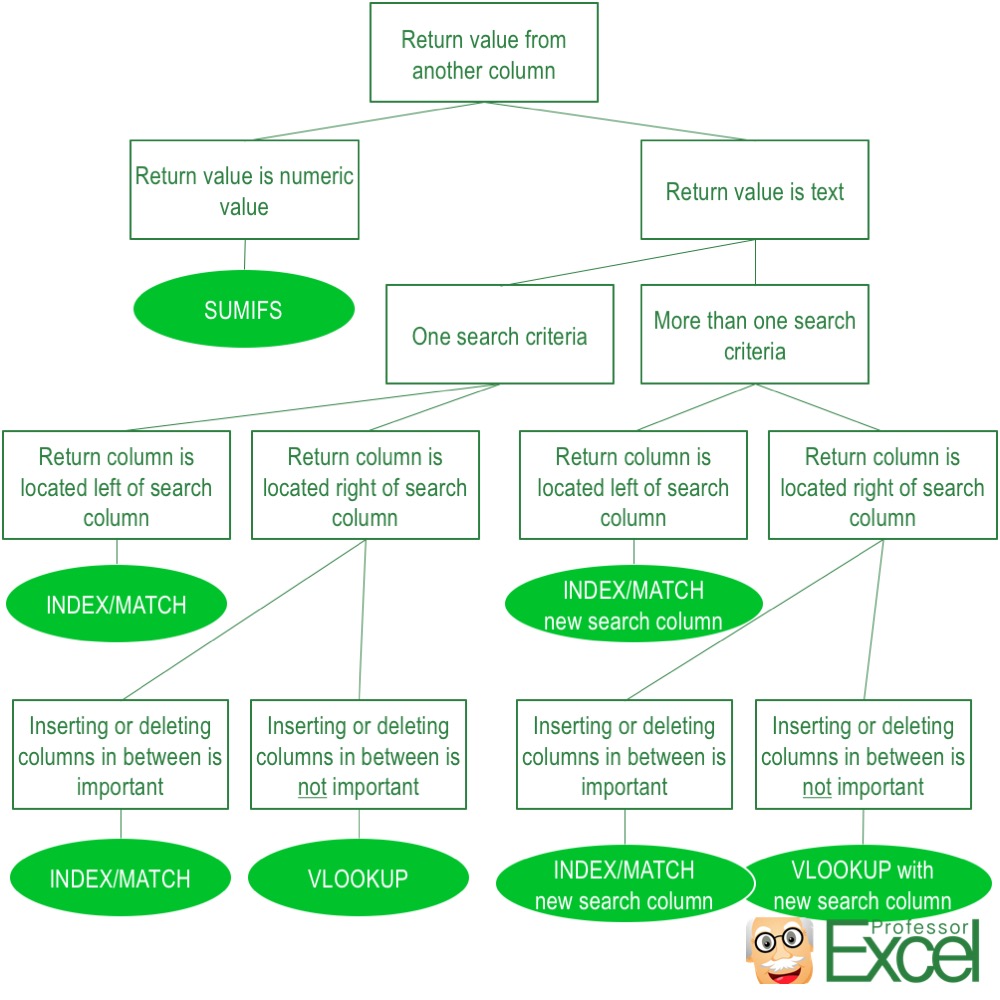
If your return value is a numeric value (like a number or date), SUMIFS has a some advantages (as shown in the table above) and we recommend using it. If you return value is text, both VLOOKUP and the INDEX-MATCH combination work. The following decisions are then no exclusion criterions but rather matters of convenience.
One more word to the case in which you got more than one search criteria and want to return text: In such case we recommend using a new search column, which combines all the search criteria. For instance, if you are searching for a person by first name and family name and want to return the address, you can concetanate first name and family name into one cell. That way you only have to search for the complete name within one column.
Situation 2: You can assume that all collaborators have access to XLOOKUP
Well, in such case it’s actually much easier:
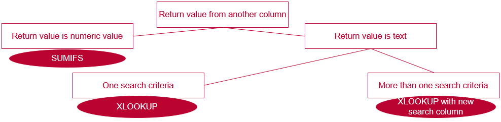
- If you have multiple search values and want to return a number, use SUMIFS.
- Otherwise, use XLOOKUP.
Performance of the lookup functions
Hold on, we haven’t talked about the calculation performance of these four lookup functions yet?
Well, this is a different topic, to my opinion. That’s why I have created separate long articles about the performance of these functions. Click here to see how is the performance of the lookup functions.
Image by Free-Photos from Pixabay
I thought index-match-match could do all the functions listed above?
You are right, index-match can do most functions as shown on the table above. But it can’t return a sum of several cells and can’t be used on several search criteria (at least not without further modifications)
I have the option of being able to use any of the formula. However, can you advise which one excel processes more easily using less memory or ram. My file is huge, so I’m trying to find alternatives and safe the space without using just values.
Hi Tina,
In such case I’d recommend either VLOOKUP or INDEX/MATCH. INDEX/MATCH is slightly faster than VLOOKUP but both formulas need half the time for calculation than SUMIFS.
For more information please refer to http://professor-excel.com/performance-excel-study/ , section “Which lookup formula is the fastest?”
Same counts for the file size, please refer to http://professor-excel.com/study-reduce-file-size-excel-workbook/#Advice_6_Use_VLOOKUP_instead_of_SUMIFS_or_INDEX-MATCH .
Best regards,
Henrik
can you help me henrik schiffner?
i have data below…
table1:
==========
ITEM | TYPE
==========
a1 | Cash
a2 | Cash
b1 | AP
c1 | AR
table2
=============
ITEM | AMOUNT
=============
a1 | 100
b1 |-100
a2 | 50
a1 | 40
b1 |-90
c1 | 200
result:
=============
TYPE | AMOUNT
=============
Cash | 190 (sumif?)
AP |-190 (sumif?)
AR | 200 (sumif?)
how do I populate a ‘sumif’ formula in the result table?
thanks & regards
hey! what about sumproduct? like
=sumproduct(RangeValue*(range1=condition 1)*(range2=condition 2)*…). it’s a lot more flexible than sumifs isn’t it?
Hi Professor,
Just one thing. The comparison table shows xlookup as NOT allowing multiple criteria.
=XLOOKUP(H5&H6&H7,B5:B15&C5:C15&D5:D15,E5:E15)
It’s easy format makes it one of it’s best features.