Advanced XLOOKUP: All the great, fancy stuff possible with XLOOKUP!

In our previous article of this big XLOOKUP series, we have explored the basic usage of XLOOKUP. Now it is time to up our game: All the great, fancy stuff you can do with XLOOKUP. We look at error catching, wildcard lookups and grouping / classification problems. These advanced XLOOKUP functions will make you the lookup master!

Overview of the big XLOOKUP series

• Part 1: Basics of XLOOKUP
• Part 2: Advanced XLOOKUP – “If not found”, “Wildcard” and “Classification” (this article)
• Part 3: 2D-XLOOKUPs
• Part 4: Let’s talk about performance of XLOOKUP
• Part 5: Convert XLOOKUP to VLOOKUP

Introduction

Also for our second part of the series, some words as an introduction.

• This article is the second part of our XLOOKUP series. If you have missed the first part describing the basics, you can find it here.
• And again, not everybody can technically use XLOOKUP yet. The reason is that it has been introduced with Excel 2019 / Office 365. Co-workers or other people working with your file might still be using Office 2016, Office 2013 or earlier versions of Excel. In fact, especially larger corporations seem to have a kind of restricted upgrade policy. So, please make sure everybody necessary can work with your file.
• The last piece of general advice: The things we are going to explore are really advanced XLOOKUP applications. Use them wisely and consider also less advanced users you collaborate with. Maybe longer but less complex solutions are sometimes better. For example, INDEX/MATCH/MATCH is still the most popular 2D lookup and SUMIFS still a great way to classify items.

Full XLOOKUP syntax

Recap first three arguments

The XLOOKUP formula can have up to six arguments. Here are the first three arguments again (for more details please refer to this article).

1. The first argument is the search or lookup value. It’s the value you look for in your Excel table.
2. The search area is a range of cells (e.g. row or column) you want to find your search value in.
3. Return area is also the range of cells you want to have a value returned from.

Advanced XLOOKUP arguments

4. IF NOT FOUND: If the search value was not found, this argument is returned. This part works similar to the IFNA function. So, if you want, you could consider the IFNA() function right inside the XLOOKUP. No need, to wrap it around any longer.
5. MATCH MODE: With the match mode you can define in what case Excel should find your search value.
   
   1. Exact match: 0 (is also the default value if you leave it blank)
   2. Get an exact match or next smaller item: -1
   3. Exact match or next larger item: 1
   4. Wildcard character match: 2
6. SEARCH MODE: The search mode determines the direction, the XLOOKUP searches for the values.
   1. The default value: Search for first-to-last: 1
   2. Search for last-to-first: -1
   3. Binary search (sorted in ascending order): 2.
      Important: this only works if you data is sorted in ascending order. If not sorted, invalid results will be returned.
   4. Binary search (sorted in descending order): -2.
      Important: this only works if you data is sorted in descending order. If not sorted, invalid results will be returned.

Advanced XLOOKUP example 1: Value not found

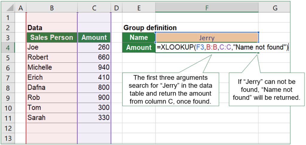
Let’s start with an easy example: You want to return “Name not found”, if a lookup value can’t be found in the search area. Assuming the following table: You have sales person names in column B and their amount sold in column C. In cell F4, you want to return the amount sold depending on the name entered in the cell above, F4.

The basic lookup is quite straight-forward:

1. Fill in the search value = F3.
   =XLOOKUP(F3,
2. Next, the search area, in this case column B. So, the second argument is “B:B”.
   =XLOOKUP(F3,B:B,
3. The third argument contains the return value, in this case the amount sold, column C.
   =XLOOKUP(F3,B:B,C:C,
4. Now, we want to extend the function to return “Name not found” in case the name was either typed incorrectly or the name is not within the list. And that’s already the forth argument – just type the return value if not found.
   =XLOOKUP(F3,B:B,C:C,“Name not found”)

Of course, a IFNA function wrapped around would serve the same purpose. But why use an additional, nested function, if XLOOKUP offers this functionality right built-in?

Advanced XLOOKUP example 2: Wildcard lookups

Our next advanced XLOOKUP example is about wildcard characters. Wildcard means that you do not specify a part of the search value (or the complete search value). For example, finding everything starting with “a”.

An example closer related to XLOOKUP: You want to search for “Victoria” but you are not sure if its written “Victoria” (with “c”) or “Viktoria” (with “k”). In such case, you could search for “Vi?toria”. So, the “Victoria” example would look like this:

Excel has two wildcard characters (“?” and “*”) as well as the tilde (“~”) in case you actually want to search for a question mark or asterisk. These characters don’t only work for XLOOKUP, but also for VLOOKUP(), any other lookup function (such as MATCH(), SUMIFS()), and the Excel search feature.

Wildcard character	Explanation
? (question mark)	Use a question mark for any single character. For example, sm?th finds “smith” and “smyth”.
* (asterisk)	Adding the asterisk finds any number of characters. For example, *east finds “Northeast” and “Southeast”.
~ (tilde) followed by ?, *, or ~	You actually want to search for the asterisk or question mark? Put a tilde in front. A question mark, asterisk, or tilde For example, fy06~? finds “fy06?”.

Explicitly specify a wildcard XLOOUP

We now know, what is a wildcard. Before we take a look at another example, there is one thing to mention: Unlike VLOOKUP, MATCH etc., you have to specify in XLOOKUP explicitly that you conduct a wildcard lookup. You do this in the SEARCH MODE argument. That means, in the fifth argument, the SEARCH MODE, you enter “2”.
If you don’t put “2” into the fifth argument and start a wildcard search, Excel conducts an exact search. That means, =XLOOKUP(“Viktoria*”,B:B,C:C) searches exactly for “Viktoria*”, including the asterisk. It is as if you’ve entered a tilde before the *.

Example for wildcard XLOOKUP

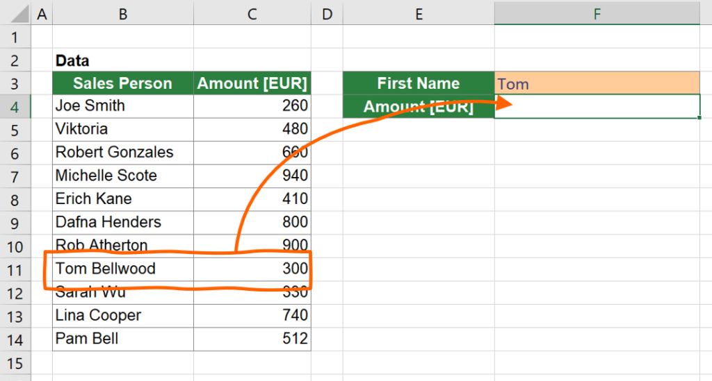
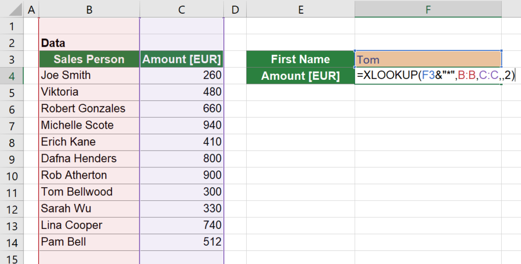
Not it’s time to finally look at a wildcard XLOOKUP example: You have a table containing sales persons with two columns, B and C. Column B has the full names, including first- and last names. The task: You only want to type the first name in cell F3 and return the amount in EUR to cell F4.

Let us set up the XLOOKUP function step-by-step:

1. The first argument is the search value. We search for the value given in cell F3, so it should be “B3″. But because we only want to type the first name and not the full name, you add &”*” to this argument.
   With the “*” you search for anything starting with “Tom”, in this case.
   =XLOOKUP(F3&”*”,
2. We search within column B, so the SEARCH AREA is B:B. You could also specify it more exact, like B4:B14, but let’s keep it simple here. =XLOOKUP(F3&”*”,B:B,
3. Return value is in column C, so the third argument is “C:C”
   =XLOOKUP(F3&”*”,B:B,C:C,
4. The fourth argument we skip here. It’s the “if not found” value and we don’t have to set it.
   =XLOOKUP(F3&”*”,B:B,C:C,,
5. And last – that’s important – we have to specify the wildcard match. So, the fifth argument has to be 2.
   =XLOOKUP(F3&”*”,B:B,C:C,,2)

Advanced XLOOKUP example 3: Group classification problem using the “next smaller item” XLOOKUP match mode

Example: Fill the group name into column D

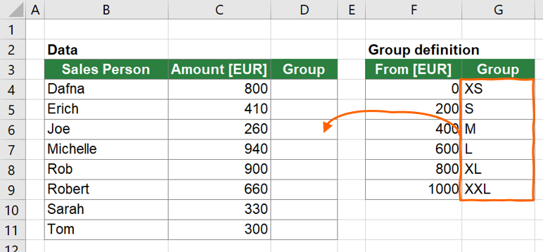
In this example, we want to classify data by its amount into groups. Let’s assume the following scenario: Depending on the sales amount in column C, you want to add the group name (e.g. XS, M, L) from column G.

So, if the amount is between 0 and 200, “XS” should be the group name. For amounts between 200 and 400, the group is “S” and so on.

The solution: Step-by-step

Again, we assemble the XLOOKUP function step-by-step for the function in cell D4.

1. The first argument is the search value. Because the classification is done by the amount, the first argument of XLOOKUP is C4.
   =XLOOKUP(C4,
2. Also, this argument should be simple: You look for the value in the cell range F4 to F9. Because we later want to copy this function down to the cells below, we right away insert $-signs in order to convert the range to an absolute reference.
   =XLOOKUP(C4,$F$4:$F$9,
3. Our desired return value should be the group name. That’s why the third argument, the return area, is the group name given in cells G4 to G9.
   =XLOOKUP(C4,$F$4:$F$9,$G$4:$G$9,
4. The forth argument defines the value if nothing can be found. We can leave it blank here.
   =XLOOKUP(C4,$F$4:$F$9,$G$4:$G$9,,
5. Now comes the trick: The fifth argument defines the “MATCH MODE”. Because we don’t search for an exact match (that would mean the value must be exactly 0, 200, 400, etc.) but rather previous, smaller value, the match mode is -1.
   To put it in slightly different words: If we search for 260 (which is not like this in the list), the return value should be “S”. So, we search for an “exact match or next smaller item”.
   =XLOOKUP(C4,$F$4:$F$9,$G$4:$G$9,,-1)

Additional comments to advanced XLOOKUP classification

• The search value is always “included”. So, if your group XS should include 200 and group S is larger than 200, you have to set up your lookup table the other way and change your lookup match mode to 1.
• Please test your function properly:
  • What happens, if you search for a value below 0 or larger than 1000?
  • Which group should be returned, if you search exactly for a group limit?
  • What happens, if you search for text?
• An alternative way for this classification problem is the SUMIFS function (check out this guide here). The advantage is that it provides slightly more options but at the same time is a bit more complex. Also, if your co-workers (or you, for that matter) don’t use newer Excel versions yet, please don’t use XLOOKUP as it’s quite new.

Download

Please download the example from above in this workbook. It also contains the basic examples from our first part of this series. Click here to start the download.